2024-07-12
한어Русский языкEnglishFrançaisIndonesianSanskrit日本語DeutschPortuguêsΕλληνικάespañolItalianoSuomalainenLatina
In the AIGC field, a special term "LoRA" frequently appears. It sounds a bit like a person's name, but it is a method of model training. LoRA stands for Low-Rank Adaptation of Large Language Models.Low-level adaptation of large language models. It is now used very frequently in stable diffusion.
Since large language models have a huge number of parameters, many large companies need to train them for several months. As a result, various training methods with lower resource consumption have been proposed, and LoRA is one of them.
This article will introduce the principles of LoRA in detail and use PyTorch to implement LoRA training for a small model.
Most model training now uses the gradient descent algorithm. The gradient descent algorithm can be divided into the following 4 steps:
Take the linear model as an example, the model parameter is W, the input and output are x and y, and the loss function is the mean square error. Then the calculation of each step is as follows. The first is forward propagation, which is a matrix multiplication for the linear model:
L=MSE(Wx,y)L = MSE(Wx, y)L=MSE(Wx,y)
After finding the loss, we can calculate the gradient of L with respect to W and get dW:
dW=∂L∂WdW = frac{partial L}{partial W}dW=∂W∂L
dW is a matrix that points to the direction where L rises fastest, but our goal is to make L decrease, so let W subtract dW. In order to adjust the pace of the update, it will also multiply a learning rate η, calculated as follows:
W′=W−ηdWW’ = W - ηdWW′=W−ηdW
Finally, repeat it all the time. The pseudo code of the above three steps is as follows:
# 4、重复1、2、3
for i in range(10000):
    # 1、正向传播计算损失
    L = MSE(Wx, y)
    # 2、反向传播计算梯度
    dW = gradient(L, W)
    # 3、利用梯度更新参数
    W -= lr * dW
After the update is completed, the new parameter W' is obtained. At this time, when we use the model to predict, the calculation is as follows:
pred=W′xpred = W’xpred=W′x
Let's think about the relationship between W and W'. W usually refers to the parameters of the basic model, while W' is obtained by adding and subtracting several matrices based on the basic model. Assuming that dW is updated 10 times during training, and each time dW is dW1, dW2, ..., dW10, then the complete update process can be written as one operation:
W′=W−ηdW1−ηdW2−…−ηdW10 Let: dW=∑i=110dWiW′=W−ηdWW' = W - ηdW_1 - ηdW_2 - … - ηdW_{10} \ Let: dW = sum_{i=1}^{10}dW_i \ W' = W - ηdW W′=W−ηdW1−ηdW2−…−ηdW10Let: dW=i=1∑10dWiW′=W−ηdW
Where dW is a matrix with the same shape as W'. We write -ηdW as a matrix R, then the updated parameters are:
W′=W+RW’ = W + RW′=W+R
At this point, the training process is simplified to the original matrix plus another matrix R. However, solving the matrix R is not simpler, and it does not save resources, so the idea of LoRA is introduced.
A well-trained matrix is usually full rank or basically satisfies the rank, that is, no column in the matrix is redundant. The paper "Scaling Laws for Neural Language Model" proposes the relationship between the dataset and the parameter size. If the relationship is satisfied and the training is good, the obtained model is basically full rank. When fine-tuning the model, we will select a base model, which is basically full rank. What about the update matrix R rank?
We assume that the R matrix is a low-rank matrix with many repeated columns, so it can be decomposed into two smaller matrices. If the shape of W is m×n, then the shape of A is also m×n. We decompose the matrix R into AB (where A is m×r and B is r×N). r is usually selected to be a value much smaller than m and n, as shown in the figure:

There are several benefits to decomposing a low-rank matrix into two matrices. First, the number of parameters is significantly reduced. Assuming that the shape of the R matrix is 100×100, the number of parameters of R is 10,000. When we choose a rank of 10, the shape of matrix A is 100×10, and the shape of matrix B is 10×100. At this time, the number of parameters is 2,000, which is 80% less than that of the R matrix.
And because R is a low-rank matrix, under sufficient training, the A and B matrices can achieve the effect of R. The matrix AB here is what we often call the LoRA model.
After the introduction of LoRA, our prediction needs to input x into W and AB respectively. At this time, the prediction calculation is:
pred=Wx+ABxpred = Wx + ABxpred=Wx+ABx
It is slightly slower than the original model when predicting, but the difference is barely noticeable in large models.
In order to grasp every detail, we do not use a large model as the actual combat of Lora, but choose to use a small network such as VGG19 to train the Lora model. Import the modules needed:
import os
import torch
from torch import optim, nn
from PIL import Image
from torch.utils import data
from torchvision import models
from torchvision.transforms import transforms
Here we use the pre-trained weights of vgg19 on imagenet as the base model, so we need to prepare a classification dataset. For convenience, only one category and 5 images are prepared here. The images are in the projectdata/goldfishDown:

Imagenet contains the goldfish category, but here we choose the illustration version of goldfish. After testing, the pre-trained model cannot correctly classify the above picture. Our goal is to train LoRA to make the model correctly classify.
We create a LoraDataset:
transform = transforms.Compose([
    transforms.Resize(256),
    transforms.CenterCrop(224),
    transforms.ToTensor(),
    transforms.Normalize(mean=[0.485, 0.456, 0.406], std=[0.229, 0.224, 0.225]),
])


class LoraDataset(data.Dataset):
    def __init__(self, data_path="datas"):
        categories = models.VGG19_Weights.IMAGENET1K_V1.value.meta["categories"]
        self.files = []
        self.labels = []
        for dir in os.listdir(data_path):
            dirname = os.path.join(data_path, dir)
            for file in os.listdir(dirname):
                self.files.append(os.path.join(dirname, file))
                self.labels.append(categories.index(dir))

    def __getitem__(self, item):
        image = Image.open(self.files[item]).convert("RGB")
        label = torch.zeros(1000, dtype=torch.float64)
        label[self.labels[item]] = 1.
        return transform(image), label

    def __len__(self):
        return len(self.files)
We encapsulate LoRA into a layer. There are only two matrices in LoRA that need to be trained. The code of LoRA is as follows:
class Lora(nn.Module):
    def __init__(self, m, n, rank=10):
        super().__init__()
        self.m = m
        self.A = nn.Parameter(torch.randn(m, rank))
        self.B = nn.Parameter(torch.zeros(rank, n))

    def forward(self, inputs):
        inputs = inputs.view(-1, self.m)
        return torch.mm(torch.mm(inputs, self.A), self.B)
Where m is the size of the input, n is the size of the output, and rank is the size of the rank, which we can set to a smaller value.
When initializing the weights, we initialize A with Gaussian noise and B with a 0 matrix to ensure that training starts from the bottom model. Because AB is a 0 matrix, LoRA does not work in the initial state.
The next step is training, which is basically the same as the regular training code of PyTorch. Let’s look at the code first:
# 加载底模和lora
vgg19 = models.vgg19(models.VGG19_Weights.IMAGENET1K_V1)
for params in vgg19.parameters():
    params.requires_grad = False
vgg19.eval()
lora = Lora(224 * 224 * 3, 1000)
# 加载数据
lora_loader = data.DataLoader(LoraDataset(), batch_size=batch_size, shuffle=True)
# 加载优化器
optimizer = optim.Adam(lora.parameters(), lr=lr)
# 定义损失
loss_fn = nn.CrossEntropyLoss()
# 训练
for epoch in range(epochs):
    for image, label in lora_loader:
        # 正向传播
        pred = vgg19(image) + lora(image)
        loss = loss_fn(pred, label)
        # 反向传播
        loss.backward()
        # 更新参数
        optimizer.step()
        optimizer.zero_grad()
        print(f"loss: {loss.item()}")
There are two points to note here. The first is that we set the weights of vgg19 to be non-trainable, which is very similar to transfer learning, but it is actually different.
The second point is that during forward propagation, we used the following code:
pred = vgg19(image) + lora(image)
Let's do a simple test:
# 测试
for image, _ in lora_loader:
    pred = vgg19(image) + lora(image)
    idx = torch.argmax(pred, dim=1).item()
    category = models.VGG19_Weights.IMAGENET1K_V1.value.meta["categories"][idx]
    print(category)
torch.save(lora.state_dict(), 'lora.pth')
The output is as follows:
goldfish
goldfish
goldfish
goldfish
goldfish
The basic prediction is correct, but this test result does not mean anything. In the end, we saved a 5M LoRA model, which is very small compared to the dozens of MB of vgg19.
LoRA is an efficient training method for large models, and this article uses LoRA in a small classification network to give readers a clearer understanding of the detailed implementation of LoRA (also because it cannot run large models). Due to the limited amount of data, the accuracy and efficiency of LoRA are not discussed in detail. Readers can refer to relevant materials for in-depth understanding.
I have worked in first-tier Internet companies for more than ten years and have mentored many colleagues and helped many people learn and grow.
I realize that there are a lot of experiences and knowledge worth sharing with everyone, and we can also use our abilities and experiences to answer many of your confusions in artificial intelligence learning, so I still insist on organizing and sharing them despite my busy work. However, due to the limited channels for knowledge dissemination, many friends in the Internet industry cannot obtain the correct information to improve their learning, so I will share important AI big model materials, including AI big model entry learning mind maps, high-quality AI big model learning books and manuals, video tutorials, practical learning and other recorded videos for free.

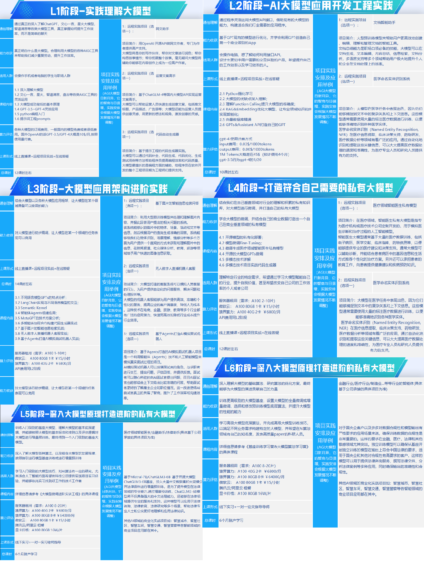
Phase 1: Starting from the design of large model system, explain the main methods of large model;
The second stage: Using the large model prompt word project to better play the role of the model from the perspective of prompts;
Phase 3: Large model platform application development uses Alibaba Cloud PAI platform to build a virtual fitting system in the e-commerce field;
Phase 4: Large model knowledge base application development, taking the LangChain framework as an example, to build an intelligent question-and-answer system for logistics industry consultation;
The fifth stage: fine-tuning and development of large models, with the help of big health, new retail, and new media to build large models suitable for the current fields;
Phase 6: Based on the SD multimodal large model, a Wenshengtu applet case was built;
The seventh stage: Focusing on the application and development of large model platforms, building large model industry applications through mature large models such as the Spark Big Model and Wenxin Big Model.

👉学会后的收获:👈
• Based on the full-stack engineering implementation of large models (front-end, back-end, product manager, design, data analysis, etc.), you can acquire different abilities through this course;
• Ability to use big models to solve relevant practical project needs: In the era of big data, more and more companies and institutions need to process massive amounts of data. Using big model technology can better process this data and improve the accuracy of data analysis and decision-making. Therefore, mastering big model application development skills can enable programmers to better respond to practical project needs;
• Based on big models and enterprise data AI application development, implement big model theory, master GPU computing power, hardware, LangChain development framework and project practical skills, learn Fine-tuning vertical training big models (data preparation, data distillation, big model deployment) in one stop;
• Ability to complete the current popular large-model vertical field model training capabilities and improve programmers’ coding capabilities: Large-model application development requires mastering technologies such as machine learning algorithms and deep learning frameworks. The mastery of these technologies can improve programmers’ coding and analytical capabilities, allowing programmers to write high-quality code more proficiently.

1. AI large model learning roadmap
2.100 sets of commercialization solutions for large AI models
3.100 large model video tutorials
4.200 large model PDF books
5.LLM interview questions collection
6. AI Product Manager Resource Collection
👉获取方式:
😝有需要的小伙伴,可以保存图片到wx扫描二v码免费领取【保证100%免费】🆓
