
내 연락처 정보
우편메소피아@프로톤메일.com
2024-07-12
한어Русский языкEnglishFrançaisIndonesianSanskrit日本語DeutschPortuguêsΕλληνικάespañolItalianoSuomalainenLatina
유전 알고리즘(GA)은 자연 선택과 유전학에서 영감을 얻은 최적화 알고리즘입니다. 1970년대 미국 학자 존 홀랜드(John Holland)가 자연 시스템의 적응성을 연구하고 컴퓨터 과학의 최적화 문제에 적용하려는 목적으로 처음 제안했습니다.
1975년: 존 홀랜드(John Holland)는 그의 저서 "Adaptation in Natural and Artificial Systems"에서 유전자 알고리즘의 개념을 처음 제안했습니다.
1980년대: 유전자 알고리즘은 기능최적화, 조합최적화 등의 분야에서 사용되기 시작하면서 점차 주목을 받게 되었다.
1990년대: 컴퓨터 컴퓨팅 성능이 향상되면서 유전 알고리즘은 공학, 경제, 생물학 및 기타 분야에서 널리 사용되었습니다.
2000년대~현재: 유전알고리즘의 이론과 응용이 더욱 발전하여 다음과 같은 다양한 개선된 알고리즘이 등장하였다.遗传编程(유전적 프로그래밍)、差分进化(미분진화) 등
유전 알고리즘은 자연 선택과 유전학을 기반으로 한 무작위 검색 방법으로, 기본 아이디어는 생물학적 진화 과정을 시뮬레이션하는 것입니다.선택하다、십자가그리고돌연변이운영은 지속적으로 새로운 세대의 인구를 생성하여 점차적으로 최적의 솔루션에 접근합니다.
초기화: 초기 모집단을 무작위로 생성합니다.
선택하다: 피트니스 기능을 바탕으로 더 나은 개인을 선택합니다.
십자가: 부모 개체의 유전자 일부를 교환하여 새로운 개체를 만듭니다.
돌연변이: 개인의 일부 유전자를 무작위로 변경합니다.
반복하다: 종료 조건이 만족될 때까지 선택, 교차, 돌연변이 과정을 반복합니다.
인구 규모를 N으로 하고 각 개체의 염색체 길이를 L로 가정합니다. 유전자 알고리즘의 수학적 과정은 다음과 같습니다.
초기화: 인구를 생성합니다. 염색체는 어디에 있습니까?
체력 계산: 개인별 체력치를 계산합니다.
선택하다: 체력 수치에 따라 개인을 선택합니다. 일반적으로 사용되는 방법에는 룰렛 선택, 토너먼트 선택 등이 있습니다.
십자가: 새로운 개체를 생성하기 위해 교차 작업을 위해 일부 개체를 선택합니다.
돌연변이: 일부 새로운 개체에 대해 돌연변이 작업을 수행하여 돌연변이 개체를 생성합니다.
인구 업데이트: 오래된 개체를 새로운 개체로 대체하여 새로운 세대의 인구를 형성합니다.
종료 조건: 미리 설정된 종료 조건(반복 횟수, 적합도 임계값 등)에 도달하면 최적의 솔루션이 출력됩니다.
유전 알고리즘은 적응성과 견고성으로 인해 많은 분야에서 널리 사용되었습니다.
구조적 최적화: 가볍고 고강도 구조로 설계되었습니다.
매개변수 최적화: 최적의 성능을 위해 시스템 매개변수를 조정합니다.
포트폴리오 최적화: 투자자산을 배분하여 수익을 극대화합니다.
시장 예측: 주가와 시장 동향을 예측합니다.
유전자 서열 비교: DNA 염기서열을 비교, 분석합니다.
단백질 구조 예측: 단백질의 3차원 구조를 예측합니다.
신경망 훈련: 신경망의 가중치와 구조를 최적화합니다.
기능 선택: 분류 또는 회귀에 가장 유리한 특성을 선택합니다.
다음 코드 예제에서는 여행하는 외판원 문제를 해결하기 위해 유전 알고리즘을 구현합니다.旅行商问题(TSP)는 여행하는 세일즈맨이 주어진 각 도시 집합을 정확히 한 번만 방문하고 궁극적으로 시작 도시로 돌아갈 수 있는 최단 경로를 찾는 것을 목표로 하는 고전적인 조합 최적화 문제입니다. 즉, 전체 이동 거리 또는 비용을 광범위하게 최소화합니다. 물류, 생산 일정 및 기타 분야에 사용됩니다.
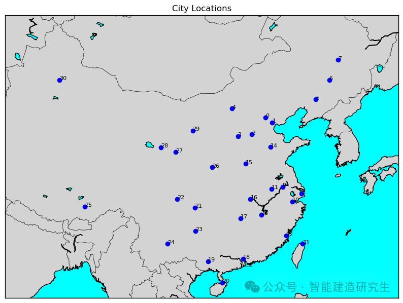
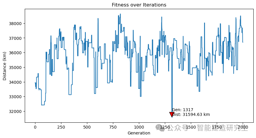
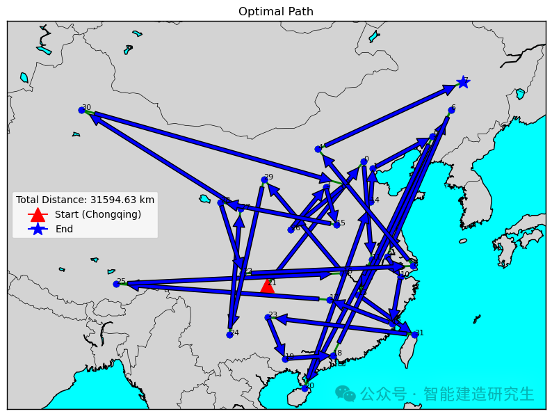
먼저 중국의 모든 지방 수도를 정의합니다(포함).중국 대만 성의 수도 타이베이) 및 해당 좌표 데이터를 사용하고哈夫曼公式두 점 사이의 거리를 계산한 후 통과遗传算法초기 모집단을 생성하고, 다음 세대를 재현, 돌연변이 및 생성하고, 지속적으로 경로를 최적화하고, 최종적으로 각 세대에서 최단 경로의 거리와 해당 경로를 기록하고, 모든 반복에서 최단 경로를 찾아 지도에 시각적으로 표시합니다.모든 도시 위치、반복 횟수에 따른 적합도 변화 최적의 경로뿐만 아니라 최종 결과는 충칭에서 모든 도시를 통과하는 최단 경로와 전체 거리를 보여줍니다. 총 2번의 훈련 시간, 첫 번째 반복 횟수는 2000, 실행 시간은 약 3분, 두 번째 반복 횟수는 20000, 실행 시간은 약 15분입니다.
한 문장으로 요약하자면, 충칭에서 시작하여 중국의 모든 성의 수도를 여행하고 유전자 알고리즘을 사용하여 최단 경로를 찾는 것입니다. 다음은 코드 구현입니다.
- import numpy as np
- import matplotlib.pyplot as plt
- from mpl_toolkits.basemap import Basemap
- import random
- from math import radians, sin, cos, sqrt, atan2
-
- # 设置随机种子以保证结果可重复
- random.seed(42)
- np.random.seed(42)
-
- # 定义城市和坐标列表,包括台北
- cities = {
- "北京": (39.9042, 116.4074),
- "天津": (39.3434, 117.3616),
- "石家庄": (38.0428, 114.5149),
- "太原": (37.8706, 112.5489),
- "呼和浩特": (40.8426, 111.7511),
- "沈阳": (41.8057, 123.4315),
- "长春": (43.8171, 125.3235),
- "哈尔滨": (45.8038, 126.5349),
- "上海": (31.2304, 121.4737),
- "南京": (32.0603, 118.7969),
- "杭州": (30.2741, 120.1551),
- "合肥": (31.8206, 117.2272),
- "福州": (26.0745, 119.2965),
- "南昌": (28.6820, 115.8579),
- "济南": (36.6512, 117.1201),
- "郑州": (34.7466, 113.6254),
- "武汉": (30.5928, 114.3055),
- "长沙": (28.2282, 112.9388),
- "广州": (23.1291, 113.2644),
- "南宁": (22.8170, 108.3665),
- "海口": (20.0174, 110.3492),
- "重庆": (29.5638, 106.5507),
- "成都": (30.5728, 104.0668),
- "贵阳": (26.6477, 106.6302),
- "昆明": (25.0460, 102.7097),
- "拉萨": (29.6520, 91.1721),
- "西安": (34.3416, 108.9398),
- "兰州": (36.0611, 103.8343),
- "西宁": (36.6171, 101.7782),
- "银川": (38.4872, 106.2309),
- "乌鲁木齐": (43.8256, 87.6168),
- "台北": (25.032969, 121.565418)
- }
-
- # 城市列表和坐标
- city_names = list(cities.keys())
- locations = np.array(list(cities.values()))
- chongqing_index = city_names.index("重庆")
-
- # 使用哈夫曼公式计算两点间的距离
- def haversine(lat1, lon1, lat2, lon2):
- R = 6371.0 # 地球半径,单位为公里
- dlat = radians(lat2 - lat1)
- dlon = radians(lon1 - lon2)
- a = sin(dlat / 2)**2 + cos(radians(lat1)) * cos(radians(lat2)) * sin(dlon / 2)**2
- c = 2 * atan2(sqrt(a), sqrt(1 - a))
- distance = R * c
- return distance
-
- # 计算路径总距离的函数,单位为公里
- def calculate_distance(path):
- return sum(haversine(locations[path[i]][0], locations[path[i]][1], locations[path[i + 1]][0], locations[path[i + 1]][1]) for i in range(len(path) - 1))
-
- # 创建初始种群
- def create_initial_population(size, num_cities):
- population = []
- for _ in range(size):
- individual = random.sample(range(num_cities), num_cities)
- # 确保重庆为起点
- individual.remove(chongqing_index)
- individual.insert(0, chongqing_index)
- population.append(individual)
- return population
-
- # 对种群进行排名
- def rank_population(population):
- # 按照路径总距离对种群进行排序
- return sorted([(i, calculate_distance(individual)) for i, individual in enumerate(population)], key=lambda x: x[1])
-
- # 选择交配池
- def select_mating_pool(population, ranked_pop, elite_size):
- # 选择排名前elite_size的个体作为交配池
- return [population[ranked_pop[i][0]] for i in range(elite_size)]
-
- # 繁殖新个体
- def breed(parent1, parent2):
- # 繁殖两个父母生成新个体
- geneA = int(random.random() * (len(parent1) - 1)) + 1
- geneB = int(random.random() * (len(parent1) - 1)) + 1
- start_gene = min(geneA, geneB)
- end_gene = max(geneA, geneB)
- child = parent1[:start_gene] + parent2[start_gene:end_gene] + parent1[end_gene:]
- child = list(dict.fromkeys(child))
- missing = set(range(len(parent1))) - set(child)
- for m in missing:
- child.append(m)
- # 确保重庆为起点
- child.remove(chongqing_index)
- child.insert(0, chongqing_index)
- return child
-
- # 突变个体
- def mutate(individual, mutation_rate):
- for swapped in range(1, len(individual) - 1):
- if random.random() < mutation_rate:
- swap_with = int(random.random() * (len(individual) - 1)) + 1
- individual[swapped], individual[swap_with] = individual[swap_with], individual[swapped]
- return individual
-
- # 生成下一代
- def next_generation(current_gen, elite_size, mutation_rate):
- ranked_pop = rank_population(current_gen)
- mating_pool = select_mating_pool(current_gen, ranked_pop, elite_size)
- children = []
- length = len(mating_pool) - elite_size
- pool = random.sample(mating_pool, len(mating_pool))
- for i in range(elite_size):
- children.append(mating_pool[i])
- for i in range(length):
- child = breed(pool[i], pool[len(mating_pool)-i-1])
- children.append(child)
- next_gen = [mutate(ind, mutation_rate) for ind in children]
- return next_gen
-
- # 遗传算法主函数
- def genetic_algorithm(population, pop_size, elite_size, mutation_rate, generations):
- pop = create_initial_population(pop_size, len(population))
- progress = [(0, rank_population(pop)[0][1], pop[0])] # 记录每代的最短距离和代数
- for i in range(generations):
- pop = next_generation(pop, elite_size, mutation_rate)
- best_route_index = rank_population(pop)[0][0]
- best_distance = rank_population(pop)[0][1]
- progress.append((i + 1, best_distance, pop[best_route_index]))
- best_route_index = rank_population(pop)[0][0]
- best_route = pop[best_route_index]
- return best_route, progress
-
- # 调整参数
- pop_size = 500 # 增加种群大小
- elite_size = 100 # 增加精英比例
- mutation_rate = 0.005 # 降低突变率
- generations = 20000 # 增加迭代次数
-
- # 运行遗传算法
- best_route, progress = genetic_algorithm(city_names, pop_size, elite_size, mutation_rate, generations)
-
- # 找到最短距离及其对应的代数
- min_distance = min(progress, key=lambda x: x[1])
- best_generation = min_distance[0]
- best_distance = min_distance[1]
-
- # 图1:地图上显示城市位置
- fig1, ax1 = plt.subplots(figsize=(10, 10))
- m1 = Basemap(projection='merc', llcrnrlat=18, urcrnrlat=50, llcrnrlon=80, urcrnrlon=135, resolution='l', ax=ax1)
- m1.drawcoastlines()
- m1.drawcountries()
- m1.fillcontinents(color='lightgray', lake_color='aqua')
- m1.drawmapboundary(fill_color='aqua')
- for i, (lat, lon) in enumerate(locations):
- x, y = m1(lon, lat)
- m1.plot(x, y, 'bo')
- ax1.text(x, y, str(i), fontsize=8)
- ax1.set_title('City Locations')
- plt.show()
-
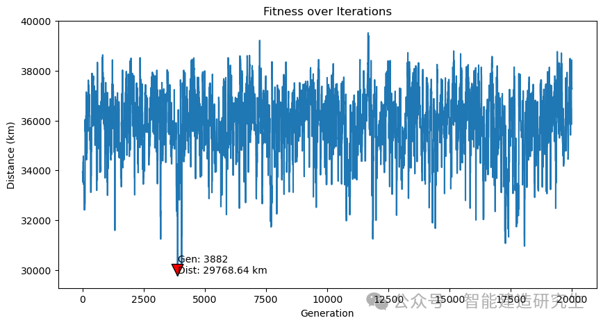
- # 图2:适应度随迭代次数变化
- fig2, ax2 = plt.subplots(figsize=(10, 5))
- ax2.plot([x[1] for x in progress])
- ax2.set_ylabel('Distance (km)')
- ax2.set_xlabel('Generation')
- ax2.set_title('Fitness over Iterations')
- # 在图中标注最短距离和对应代数
- ax2.annotate(f'Gen: {best_generation}nDist: {best_distance:.2f} km',
- xy=(best_generation, best_distance),
- xytext=(best_generation, best_distance + 100),
- arrowprops=dict(facecolor='red', shrink=0.05))
- plt.show()
-
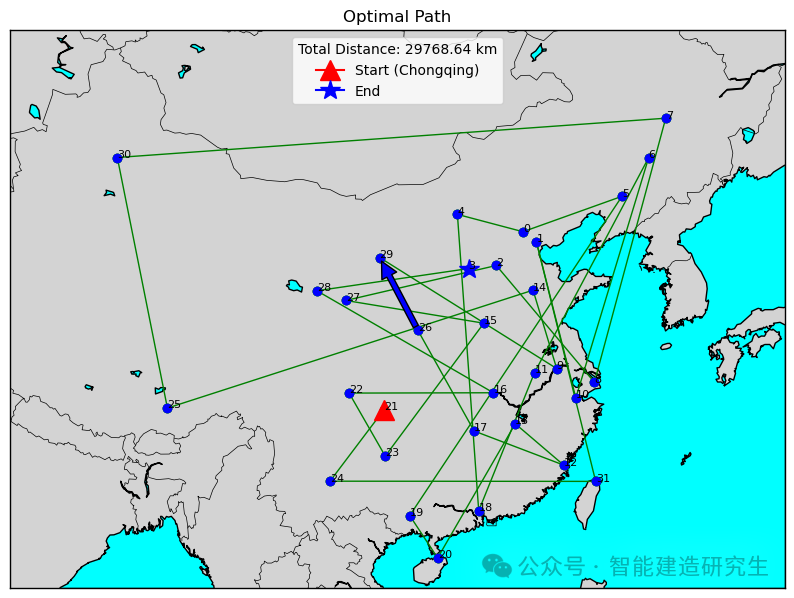
- # 图3:显示最优路径
- fig3, ax3 = plt.subplots(figsize=(10, 10))
- m2 = Basemap(projection='merc', llcrnrlat=18, urcrnrlat=50, llcrnrlon=80, urcrnrlon=135, resolution='l', ax=ax3)
- m2.drawcoastlines()
- m2.drawcountries()
- m2.fillcontinents(color='lightgray', lake_color='aqua')
- m2.drawmapboundary(fill_color='aqua')
-
- # 绘制最优路径和有向箭头
- for i in range(len(best_route) - 1):
- x1, y1 = m2(locations[best_route[i]][1], locations[best_route[i]][0])
- x2, y2 = m2(locations[best_route[i + 1]][1], locations[best_route[i + 1]][0])
- m2.plot([x1, x2], [y1, y2], color='g', linewidth=1, marker='o')
-
- # 只添加一个代表方向的箭头
- mid_index = len(best_route) // 2
- mid_x1, mid_y1 = m2(locations[best_route[mid_index]][1], locations[best_route[mid_index]][0])
- mid_x2, mid_y2 = m2(locations[best_route[mid_index + 1]][1], locations[best_route[mid_index + 1]][0])
- ax3.annotate('', xy=(mid_x2, mid_y2), xytext=(mid_x1, mid_y1), arrowprops=dict(facecolor='blue', shrink=0.05))
-
- # 在最优路径图上绘制城市位置
- for i, (lat, lon) in enumerate(locations):
- x, y = m2(lon, lat)
- m2.plot(x, y, 'bo')
- ax3.text(x, y, str(i), fontsize=8)
-
- # 添加起点和终点标记
- start_x, start_y = m2(locations[best_route[0]][1], locations[best_route[0]][0])
- end_x, end_y = m2(locations[best_route[-1]][1], locations[best_route[-1]][0])
- ax3.plot(start_x, start_y, marker='^', color='red', markersize=15, label='Start (Chongqing)') # 起点
- ax3.plot(end_x, end_y, marker='*', color='blue', markersize=15, label='End') # 终点
-
- # 添加总距离的图例
- ax3.legend(title=f'Total Distance: {best_distance:.2f} km')
-
- ax3.set_title('Optimal Path')
- plt.show()
-
중국의 모든 지방 수도의 위치 시각화:
반복 횟수는 2,000입니다(최단 거리는 31594km).
과거 반복 과정에서 최단 경로의 반복을 찾아 최단 경로를 시각화합니다.
사례 2: 반복 횟수는 20,000입니다(구한 최단 거리는 29,768km입니다).
과거 반복 프로세스에서 최단 경로가 있는 반복을 찾고 해당 반복에 대한 최단 경로를 시각화합니다.
위 내용은 인터넷에서 요약한 내용입니다. 도움이 되셨다면 다음에 또 만나요!

그는 30년 이상 기술 연구에 전념해 왔으며, java, linux, javascript, php, css 등 다양한 언어에 능숙하며, 오픈 소스 분야에 많은 공헌을 했습니다. 나중에 참조할 수 있도록 기술 개발의 일부 문제를 공유하는 개발자 문서 스테이션입니다.

우편메소피아@프로톤메일.com