Technology Sharing

한어Русский языкEnglishFrançaisIndonesianSanskrit日本語DeutschPortuguêsΕλληνικάespañolItalianoSuomalainenLatina

1. Introduction to classification based on probabilistic neural network (PNN)

PNN (Probabilistic Neural Network) is a neural network model based on probability theory, mainly used to solve classification problems. PNN was first proposed by Makovsky and Masikin in 1993 and is a very effective classification algorithm.

The principle of PNN can be simply summarized into the following steps:

1. Data input layer: Input the sample data into the model respectively.
2. Mode layer:Perform pattern matching on each input data and calculate the similarity score between it and the specified category.
3. Mode comparison layer:The similarity scores of all categories are compared, and the category with the highest score is found as the final classification result.

PNN has the following characteristics:

1. Efficiency: PNN has a fast training speed and shows high classification accuracy in practical applications.
2. robustness:PNN is highly robust to noise and outliers and can effectively handle complex classification problems.
3. Easy to explain:The results of PNN can be explained intuitively, allowing users to better understand the classification basis of the model.

In general, PNN is a very effective classification algorithm, which is suitable for classification problems in various fields, such as image recognition, text classification, etc.

2. Classification description and key functions based on probabilistic neural network (PNN)

1) Description

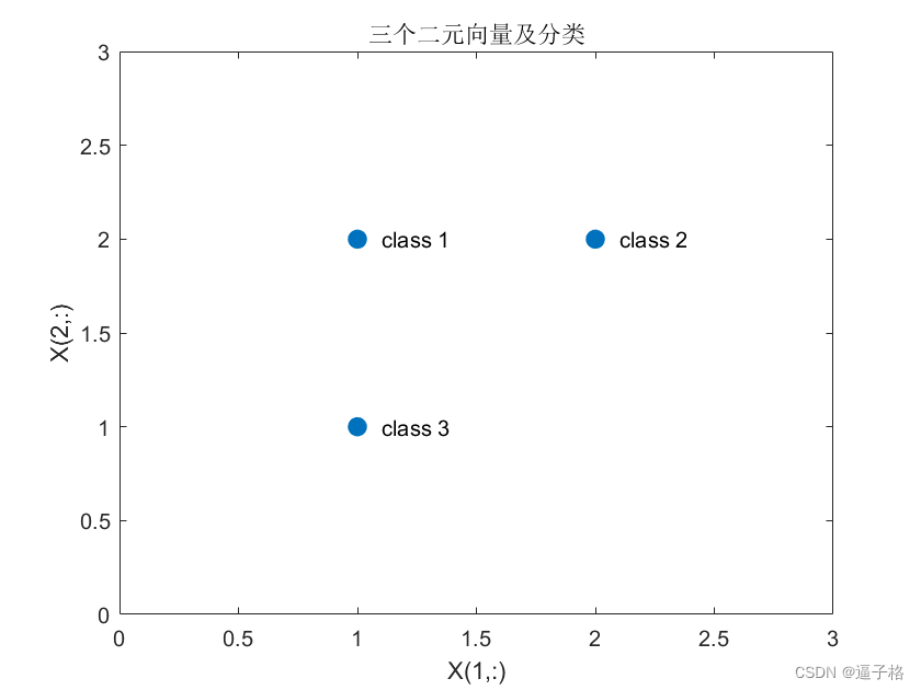
Here there are three binary input vectors X and their associated classes Tc.
Create y probabilistic neural network that correctly classifies these vectors.

2) Important functions

newpnn() function:Designing a probabilistic neural network

Probabilistic Neural Network (PNN) is a radial basis network suitable for classification problems.

grammar

net = newpnn(P,T,spread)% Accepts two or three parameters and returns a new probabilistic neural network.

parameter

P：r × Q matrix of Q input vectors

T：s × Q matrix of Q target class vectors

spread: Spread of radial basis functions (default = 0.1)

If the spread is close to zero, the network acts as a nearest neighbor classifier. When the spread becomes larger, the designed network considers several nearby design vectors.

sim() function: simulate neural network

grammar

[Y,Xf,Af] = sim(net,X,Xi,Ai,T) 
parameter

net: network

X: Network input

Xi: Initial input delay condition (default = 0)

Ai: Initial layer delay condition (default = 0)

T: Network target (default = 0)

3. Dataset and display

Code

X = [1 2; 2 2; 1 1]';
Tc = [1 2 3];
figure(1)
plot(X(1,:),X(2,:),'.','markersize',30)
for i = 1:3, text(X(1,i)+0.1,X(2,i),sprintf('class %g',Tc(i))), end
axis([0 3 0 3])
title('三个二元向量及分类')
xlabel('X(1,:)')
ylabel('X(2,:)')

View Effects

4. Test the network based on the designed input vector

1) Description

Convert the target class index Tc to a vector T
Designing Probabilistic Neural Networks with NEWPNN
SPREAD value is 1 because this is the typical distance in y between the input vectors.

2) Test network

Code

T = ind2vec(Tc);
spread = 1;
net = newpnn(X,T,spread);
%测试网络
%基于输入向量测试网络。通过对网络进行仿真并将其向量输出转换为索引来实现目的。
Y = net(X);
Yc = vec2ind(Y);
figure(2)
plot(X(1,:),X(2,:),'.','markersize',30)
axis([0 3 0 3])
for i = 1:3,text(X(1,i)+0.1,X(2,i),sprintf('class %g',Yc(i))),end
title('测试网络')
xlabel('X(1,:)')
ylabel('X(2,:)')

View Effects

3) Test the network with new data

Code

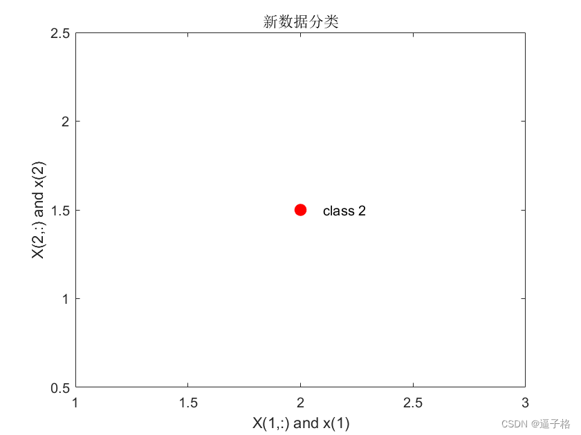
x = [2; 1.5];
y = net(x);
ac = vec2ind(y);
hold on
figure(3)
plot(x(1),x(2),'.','markersize',30,'color',[1 0 0])
text(x(1)+0.1,x(2),sprintf('class %g',ac))
hold off
title('新数据分类')
xlabel('X(1,:) and x(1)')
ylabel('X(2,:) and x(2)')

View Effects

5. The probabilistic neural network divides the input space into three classes.

illustrate

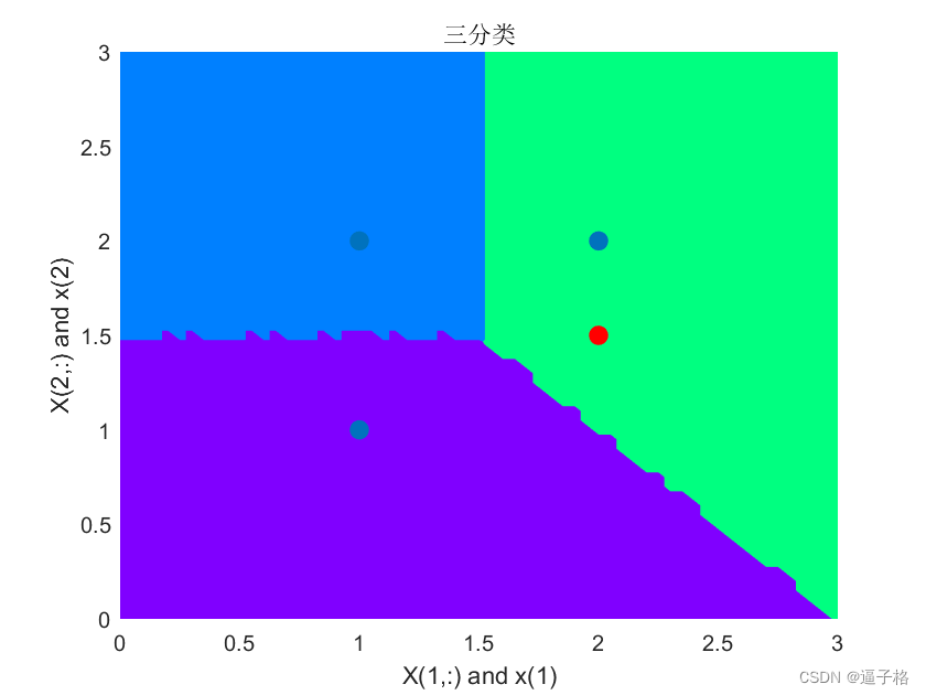
Divided into three categories

Code

x1 = 0:.05:3;
x2 = x1;
[X1,X2] = meshgrid(x1,x2);
xx = [X1(:) X2(:)]';
yy = net(xx);
yy = full(yy);
m = mesh(X1,X2,reshape(yy(1,:),length(x1),length(x2)));
m.FaceColor = [0 0.5 1];
m.LineStyle = 'none';
hold on
m = mesh(X1,X2,reshape(yy(2,:),length(x1),length(x2)));
m.FaceColor = [0 1.0 0.5];
m.LineStyle = 'none';
m = mesh(X1,X2,reshape(yy(3,:),length(x1),length(x2)));
m.FaceColor = [0.5 0 1];
m.LineStyle = 'none';
plot3(X(1,:),X(2,:),[1 1 1]+0.1,'.','markersize',30)
plot3(x(1),x(2),1.1,'.','markersize',30,'color',[1 0 0])
hold off
view(2)
title('三分类')
xlabel('X(1,:) and x(1)')
ylabel('X(2,:) and x(2)')

Try the effect

6. Summary

Probabilistic neural network (PNN) is an artificial neural network used for pattern classification. It is based on Bayes' theorem and Gaussian mixture model and can be used to process various types of data, including continuous data and discrete data. PNN is more flexible than traditional neural networks in handling classification problems and has higher accuracy and generalization ability.

The basic working principle of PNN is to calculate the similarity between the input data set and each sample in the sample set, and classify the input data according to the similarity. PNN consists of four layers: input layer, pattern layer, competition layer and output layer. The input data is first passed to the pattern layer through the input layer, then the similarity is calculated through the competition layer, and finally classified in the output layer according to the similarity.

In Matlab, you can use the relevant toolbox or program it yourself to implement PNN classification. First, you need to prepare a training data set and a test data set, and then train the PNN model with the training data set. After the training is completed, you can use the test data set to evaluate the classification performance of the PNN and make predictions.

In general, PNN is a powerful classification method that is suitable for various classification problems. In practical applications, appropriate features and model parameters can be selected according to specific problems to improve classification performance. Matlab provides a wealth of tools and function support, making the implementation and application of PNN more convenient.

7. Source code

Code

%% 基于概率神经网络(PNN)的分类(matlab)
%此处有三个二元输入向量 X 和它们相关联的类 Tc。
%创建 y 概率神经网络，对这些向量正确分类。
%重要函数：NEWPNN 和 SIM 函数
%% 数据集及显示
X = [1 2; 2 2; 1 1]';
Tc = [1 2 3];
figure(1)
plot(X(1,:),X(2,:),'.','markersize',30)
for i = 1:3, text(X(1,i)+0.1,X(2,i),sprintf('class %g',Tc(i))), end
axis([0 3 0 3])
title('三个二元向量及分类')
xlabel('X(1,:)')
ylabel('X(2,:)')
%% 基于设计输入向量测试网络
%将目标类索引 Tc 转换为向量 T
%用 NEWPNN 设计 y 概率神经网络
% SPREAD 值 1，因为这是输入向量之间的 y 典型距离。
T = ind2vec(Tc);
spread = 1;
net = newpnn(X,T,spread);
%测试网络
%基于输入向量测试网络。通过对网络进行仿真并将其向量输出转换为索引来实现目的。
Y = net(X);
Yc = vec2ind(Y);
figure(2)
plot(X(1,:),X(2,:),'.','markersize',30)
axis([0 3 0 3])
for i = 1:3,text(X(1,i)+0.1,X(2,i),sprintf('class %g',Yc(i))),end
title('测试网络')
xlabel('X(1,:)')
ylabel('X(2,:)')
%数据测试
x = [2; 1.5];
y = net(x);
ac = vec2ind(y);
hold on
figure(3)
plot(x(1),x(2),'.','markersize',30,'color',[1 0 0])
text(x(1)+0.1,x(2),sprintf('class %g',ac))
hold off
title('新数据分类')
xlabel('X(1,:) and x(1)')
ylabel('X(2,:) and x(2)')
%% 概率神经网络将输入空间分为三个类。
x1 = 0:.05:3;
x2 = x1;
[X1,X2] = meshgrid(x1,x2);
xx = [X1(:) X2(:)]';
yy = net(xx);
yy = full(yy);
m = mesh(X1,X2,reshape(yy(1,:),length(x1),length(x2)));
m.FaceColor = [0 0.5 1];
m.LineStyle = 'none';
hold on
m = mesh(X1,X2,reshape(yy(2,:),length(x1),length(x2)));
m.FaceColor = [0 1.0 0.5];
m.LineStyle = 'none';
m = mesh(X1,X2,reshape(yy(3,:),length(x1),length(x2)));
m.FaceColor = [0.5 0 1];
m.LineStyle = 'none';
plot3(X(1,:),X(2,:),[1 1 1]+0.1,'.','markersize',30)
plot3(x(1),x(2),1.1,'.','markersize',30,'color',[1 0 0])
hold off
view(2)
title('三分类')
xlabel('X(1,:) and x(1)')
ylabel('X(2,:) and x(2)')