Technology Sharing

한어Русский языкEnglishFrançaisIndonesianSanskrit日本語DeutschPortuguêsΕλληνικάespañolItalianoSuomalainenLatina

Previous section,Through the derivation of SVPWM, we have obtained the ability to control any force on the motor rotor.,In this section, we use the SVPWM form of rotor dq axis decoupling obtained in the previous section,,to reasonably control the rotor force and achieve the ultimate goal of FOC motor control:,position, speed, and current control.

PID Control

Those who read this section are most likely familiar with PID (Proportional, Integral, Derivative) control. Due to my limited ability, I will not give a complete explanation here, nor will I involve advanced control methods.
Whether it is the position, speed or current of the motor, it can be regarded as a controlled parameter.
From an intuitive point of view, when the real-time value of a controlled parameter is less than the target value, an external force needs to be applied to increase the controlled parameter. If the applied external force is too large, the controlled parameter will be over-adjusted, resulting in an increasingly large oscillation amplitude of the controlled parameter near the target value; if the applied external force is too small, the speed at which the parameter reaches the target value is too slow. Therefore, a suitable external force is needed so that the controlled parameter will not oscillate more and more violently, and the adjustment speed will not be too slow. This intuitive control idea is the P in PID. When using P control alone, the external force size is set = the difference between the controlled parameter and the target value * P coefficient. The larger the difference, the greater the external force applied, which is very intuitive. If the P coefficient is set relatively small, although the controlled parameter will not oscillate all the time and can slowly stabilize to the target value, the adjustment speed is too slow. At this time, the D control of PID can be added to make the originally oscillating controlled parameter quickly shrink to the target value.
Let's think about D control from an intuitive point of view. When the controlled parameter approaches and passes the target value under pure P control, a corrective force in the opposite direction of the speed helps the controlled parameter to brake near the target value, allowing the controlled parameter to shrink to the target value faster. This corrective force in the opposite direction of the speed is D control. After adding D control, the size of the controlled external force = the difference between the controlled parameter and the target value * P coefficient controlled parameter speed * D coefficient. When pure D control is used, since the speed of the controlled parameter is 0 in the initial state, the controlled parameter will not receive external force. It can be seen from this that P control provides external force and D control constrains external force. If the D coefficient is too large, a slight speed can cause a huge external force; if the D coefficient is too small, it is not enough to constrain the external force produced by P control, and the controlled parameter will be slow to stabilize.
Let's think about I control intuitively. When the controlled parameter is under load, the external force provided by the simple P control may not be enough to support the load. Therefore, a mechanism can be added to accumulate the difference between the controlled parameter and the target value over time, so that the power required for the controlled parameter to reach the target value when there is a load can be obtained. This mechanism is I control. After adding I control, the size of the control external force = the difference between the controlled parameter and the target value * P coefficient controlled parameter speed * D coefficient the difference between the controlled parameter and the target value accumulated over time * I coefficient.
When controlling the motor, without special circumstances, since the d-axis does not contribute to the motor rotation, PID control can only control the force of the q-axis. The d-axis can be controlled or the output can be directly set to 0.

Filtering

In speed control and current control, due to the limitations of sampling accuracy and frequency, the speed and current are unstable and change quickly. For example, the figure below is the direct calculation value of the motor speed. There are many sawtooth values, which fluctuate around the true value. If such a value is used directly, the PID output will fluctuate greatly.

The following figure is closer to the true value after filtering:There are many filtering methods, such as low-pass filtering and Kalman filtering. The essence is to estimate a value close to the truth in the data mixed with noise. Since filtering is a very large topic, the principle is not explained in this section. You can directly view the code in the subsequent practice part. Just remind you that filtering calculation is required before entering the PID controller.

Individual position control

Position refers to the angle. Please note that there are two physical angles, one is the motor angle and the other is the rotor angle, which are different. The motor encoder is installed on the rotor housing, so the encoder obtains the angle of the rotor housing, and the rotor is located inside. Since the rotor housing and the rotor are fixed to each other, there is a fixed offset between the two angles. When installing, the encoder zero degree cannot be exactly facing the rotor permanent magnet. The encoder angle is provided by the encoder, and the rotor angle can also be known. In the subsequent practical part, it will be explained how to obtain this fixed offset. In this section, you only need to complete the theoretical calculation part. The synthesized magnetic vector acts on the rotor permanent magnet, so the theoretical calculation is calculated based on the rotor angle.

There are two ways to achieve rotor position control:

pid method:
The intuitive idea is to use the rotor q-axis to continuously pull the rotor left and right. Once the rotor deviates from the target position, a reverse force is applied to the q-axis to pull it. The greater the deviation, the greater the pulling force, so that the rotor returns to the target position.
Advantages: The q-axis can provide greater force, and the position control is relatively fast and powerful.
Disadvantages: Since the q-axis is 90 degrees away from the magnetic vector of the rotor permanent magnet, the real-time position (angle) of the rotor needs to be known.
Since the real-time position of the rotor is easy to obtain with an encoder, PID position control is used in most cases.

The FOC control block diagram of a single position is shown below. The meaning of the figure is to input a target position, calculate the difference with the angle calculated by the encoder, and then input it into the pid controller to control only the q-axis strength of the rotor, and directly set the d-axis strength to 0. Finally, the dq-axis strength (between 0 and 1) is input into the SVPWM function derived in the previous article, and the PWM duty cycle of the uvw bridge arm is output. It should be noted here that the input target position${\theta }_{in}$It can be the rotor angle, encoder angle or multi-turn angle, as long as it is consistent with the feedback$\theta$Just keep the same angle.

D-axis strong drag:
The core idea is to artificially control the coil to generate a target coil magnetic vector, and the d-axis of the permanent magnet will be attracted to the target position. Note that this method attracts the d-axis to the target position.
Advantages: Since the target position is generated, there is no need to know the rotor angle, and the rotor will be attracted naturally.
Disadvantages: The tangential force component is small, and a slight tangential external force can cause the rotor to obviously move out of position.

Individual speed control

The speed control method using the D-axis dragging method is not suitable, because the D-axis dragging is to avoid using the encoder, and it is difficult to calculate the speed without the encoder data. The speed control method can be used for PID control, but since the speed value changes relatively unstable during the rotation of the motor, and D control is proportional to the degree of change of the controlled parameter, generally only PI control is used.
The calculation method of speed is very simple, that is$\frac{Current\; angle-Last\; recorded\; angle}{\Delta t}$。
Speed ​​control can be achieved by inputting the difference between the target speed and the real-time speed into the PI control.
The FOC control block diagram of a single speed is shown below.

Individual current control

The current of the motor represents the torque. After the dq axis is decoupled, it can be found that only the q axis contributes to the rotation of the motor and only the q axis generates torque. Therefore, it is only necessary to control the q axis current to control the motor torque. If the d axis current is also controlled, the motor current utilization rate can be improved, heat generation can be reduced, and the maximum torque output of the motor can be increased.

Get the motor current:
The rotor dq axis is an abstract concept for the convenience of decoupling the rotor force. The dq axis current cannot be directly detected. The current that can be directly detected is the current in the motor phase line circuit. The dq axis current can be calculated based on the phase line current.
There are many ways to detect phase line current. The two most common methods are: 1. The current detection is placed between the upper and lower bridge arm power tubes, which is called online detection. 2. The current detection is placed between the lower bridge arm and GND, which is called low-end detection.

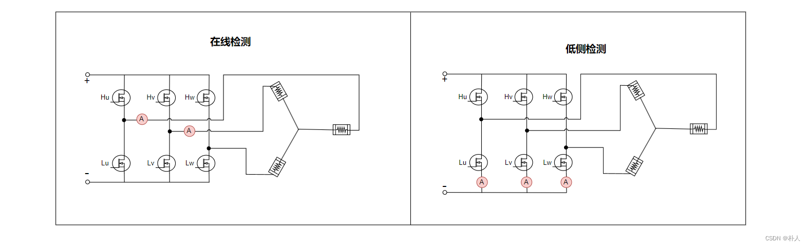
Since a node流出电流 流入电流=0, so only two current detection units are needed for three phase lines. However, it is better to use three current detection units for low-side detection, because when the PWM duty cycle of a bridge arm is 1 or close to 1, the lower bridge arm will have no current or the current will be unstable, and only one current detection unit will be left for the three phase lines to collect current normally. With three current detection units, all three can read the current, and two of the current values ​​can be selected according to the duty cycle, and the other one is calculated by the sum of the current being 0. Online detection does not have this problem, because no matter whether the lower bridge arm is in the closed state, there is always current passing through the phase line. Since the voltage at the online detection position is relatively large, the current detection unit for online detection needs to be able to withstand a large voltage, and the price is relatively high.

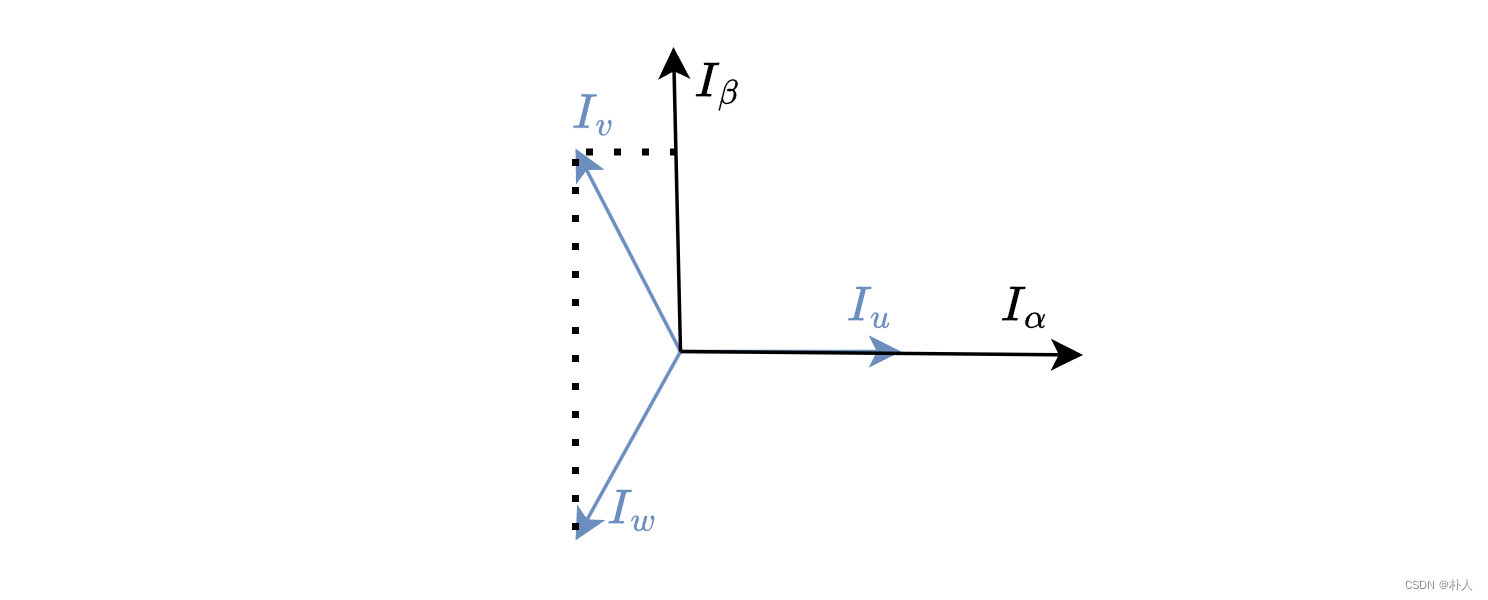
After obtaining the three phase line currents, the next step is to find a way to convert them into dq axis currents. The phase line currents can be projected onto the dq axis, so that the dq axis currents can be directly obtained. However, the current mainstream approach is to project the dq axis onto$\alpha$Axis and$\beta$axis (this step is called Clark transformation), and then$\alpha$Axis and$\beta$The axis current is projected onto the dq axis (this step is called park transformation), because it will be used in more advanced sensorless FOC.$\alpha$Axis and$\beta$Shaft current.

Clark transformation:
The three-phase current$I_u,I_v,I_w$Project to$I_{\alpha },I_{\beta }$From the geometric relationship in the figure below, we can see that the projection expression is:
$$\{\begin{array}{l}{I}_{\alpha }=I_u-I_v\ast \cos 60^{°}-I_w\ast \cos 60^{°}\\ I_{\beta }=I_v\ast \cos 30^{°}-I_w\ast \cos 30^{°}\end{array}$$

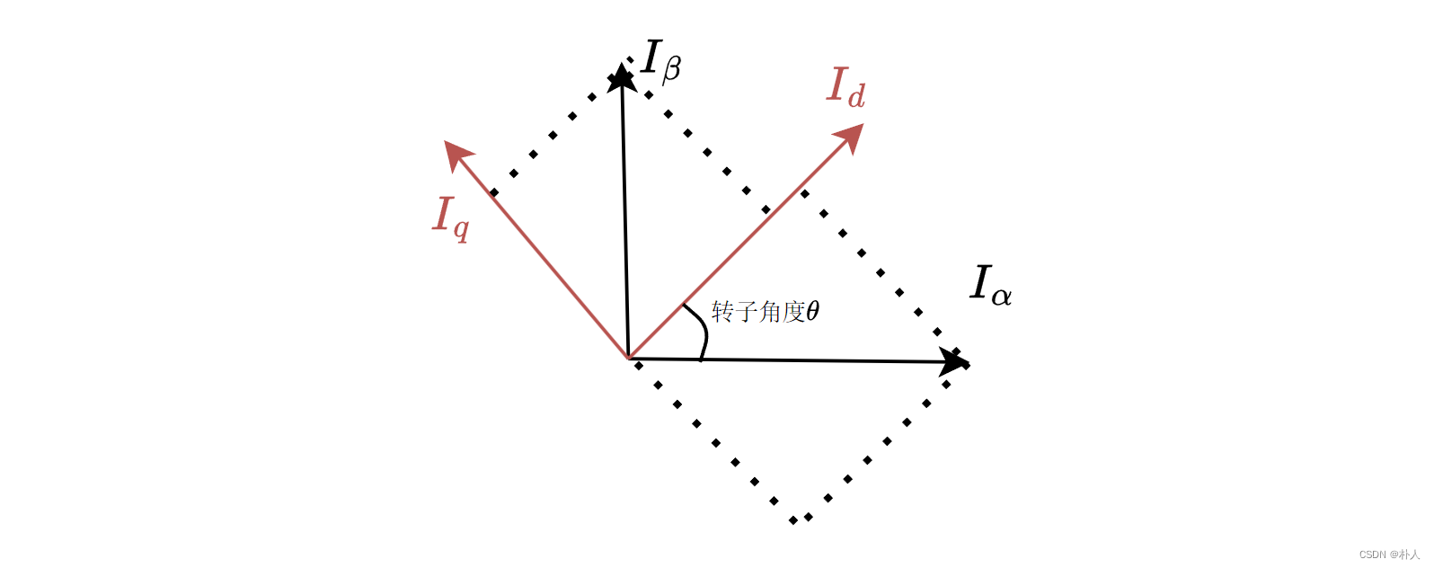
park transformation:
Will$I_{\alpha },I_{\beta }$The axis is projected onto the dq axis (actually multiplied by a rotation matrix). From the geometric relationship in the figure below, we can see that the projection expression is:
$$\{\begin{array}{l}{I}_d=I_{\alpha }\ast \cos \theta I_{\beta }\ast \sin \theta \\ I_q=-I_{\alpha }\ast \sin \theta I_{\beta }\ast \cos \theta \end{array}$$

The FOC control diagram of a single current is shown below. Since the current change is relatively unstable, the D control related to the speed of change of the controlled parameter is usually not used here, and only PI control is used.

Position-speed-current cascade control

If there is a requirement: when controlling the position, specify the maximum speed and maximum current of the motor during the homing process; or when controlling the speed, specify the maximum current of the motor during the process of reaching the target speed, then position-speed-current cascade control is required. The cascade control here does not control the motor to reach a certain current value or speed value, but requires the maximum current value or maximum speed value that the motor can reach during the control process, because it is impossible to keep the motor in one position and still have speed or current.
Cascade control means that the input of the current control loop is the output of the previous control loop. Taking cascade position control as an example, the control block diagram is:

---

The theoretical part ends here. We have obtained the calculation method of SVPWM and the control process of position, speed and current. We can write FOC code, but we will encounter various problems in practice, such as the order of phase lines, how to implement PWM duty cycle, current sampling time, peripheral configuration, etc. The next practical part uses the super common MCU with the best cost performance: smt32f103c8t6 and stm32cube tools, without using the motor library, to realize complete FOC control from scratch.