Technology Sharing

한어Русский языкEnglishFrançaisIndonesianSanskrit日本語DeutschPortuguêsΕλληνικάespañolItalianoSuomalainenLatina

• easy-rl PDF version notes organization P5, P10 - P12
• joyrl Compare and supplement P11 - P13
• OpenAI document compilation ⭐ https://spinningup.openai.com/en/latest/index.html

Download the latest version PDF
Address: https://github.com/datawhalechina/easy-rl/releases
Domestic address (recommended for domestic readers)：
Link: https://pan.baidu.com/s/1isqQnpVRWbb3yh83Vs0kbw Extraction code: us6a

easy-rl online version link (for copying code)
Reference link 2: https://datawhalechina.github.io/joyrl-book/

other:
【Correction record link】
——————
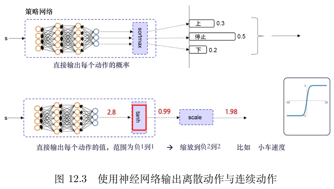
5. Basics of Deep Reinforcement Learning⭐️
Open source content: https://linklearner.com/learn/summary/11
——————————

Image Source

Proximal policy optimization (PPO)

Same-policy: The agent to learn and the agent that interacts with the environment are the same.
Off-policy: The agent to learn and the agent interacting with the environment are different

Policy Gradient: It takes a lot of time to sample data

Same strategy $\stackrel{Importance\; Sampling}{⟹}$ Different strategies

PPO: Avoid two distributions that differ too much. Same strategy algorithm
1. Original optimization items$J(\theta ,{\theta }^{\prime })$
2. Constraints:$\theta$ and${\theta }^{\prime }$ The KL divergence of the output action ($\theta$ and${\theta }^{\prime }$ The more similar the better)

PPO has a predecessor: trust region policy optimization (TRPO)
TRPO is difficult to handle because it treats the KL divergence constraint as an additional constraint and does not put it in the objective function, so it is difficult to calculate. Therefore, we generally use PPO instead of TRPO. The performance of PPO and TRPO is similar, but PPO is much easier to implement than TRPO.

KL divergence: the distance of the actions.The probability distribution of performing an action distance.

There are two main variants of the PPO algorithm: Proximal Policy Optimization Penalty (PPO-penalty) and Proximal Policy Optimization Clipping (PPO-clip).

——————————
P10 Sparse Reward Problem
1. Design rewards. Domain knowledge required
How about distributing the final reward to each relevant action?

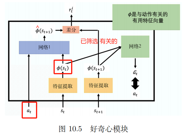
2. Curiosity
Intrinsic curiosity module (ICM)
enter:$a_t,s_t$
Output:${\hat{s}}_{t+1}$
The network's predicted value${\hat{s}}_{t+1}$ With the true value$s_{t+1}$ The more dissimilar,$r_t^i$ The bigger

$r_t^i$ ： The more difficult it is to predict the future state, the greater the reward for the action. Encourage risk-taking and exploration.

• The indicator is too single, and you may only learn useless things.

Feature extractor

Network 2:
Input: Vector$\mathbf{\varphi }(s_t)$ and$\mathbf{\varphi }(s_{t+1})$

Predicting Actions $\hat{a}$ The closer to the real action the better.

3. Course study

Easy -> Difficult

Reverse curriculum learning:
Starting from the final most ideal state (which we call the gold state), go toFind the state closest to the golden stateAs the "ideal" state that we want the intelligent agent to reach at certain stages. Of course, we will intentionally remove some extreme states in the process, that is, states that are too simple or too difficult.

4. Hierarchical reinforcement learning (HRL)
The agent's strategies are divided into high-level strategies and low-level strategies. The high-level strategy determines how to execute the low-level strategy based on the current state.

————————
P11 Imitation Learning
Unclear about the reward scenario

Imitation learning (IL)
Learning from demonstration
Apprenticeship learning
Learning by watching

There are clear rewards: board games, video games
No clear reward: Chatbots

Collect expert demonstrations: recordings of human driving, human conversations

Conversely, what kind of reward function makes the experts take these actions?
Inverse reinforcement learning isFirst find the reward function, after finding the reward function, we use reinforcement learning to find the optimal actor.

Third person imitation learning technology

————————
P12 Deep deterministic policy gradient (DDPG)

Used experience replay strategy

Ablation experiment [Control variable method] analysisEach constraintThe impact on the outcome of the battle.

---

joyrl：

DDPG_Continuous

In needDeterminismStrategy andContinuous ActionUnder the premise of space, this type of algorithm will be a relatively stable baseline algorithm

DQN in Continuous Action Space

Deep deterministic policy gradient (DDPG)

The experience replay mechanism can reduce the correlation between samples, improve the effective utilization of samples, and increase the stability of training.

shortcoming:
1. Cannot be used in discrete action spaces
2、Highly dependent on hyperparameters
3. Highly sensitive initial conditions. Affects the convergence and performance of the algorithm
4. It is easy to fall into local optimum.

• Due to the use of deterministic strategies, the algorithm may fall into local optimality and it is difficult to find the global optimal strategy. In order to increase the exploration, some measures need to be taken, such as adding noise strategies or using other exploration methods.

The advantage of soft update is that it is smoother and slower, which can avoid shocks caused by too rapid weight updates and reduce the risk of training divergence.

Twin delayed DDPG (TD3)

Double-delayed deterministic policy gradient algorithm

Three improvements: dual Q network, delayed update, noise regularization
Double Q Network: Two Q networks, choose the one with smaller Q value. This can solve the problem of overestimation of Q value and improve the stability and convergence of the algorithm.

Delayed updates: make the actor update frequency lower than the critic update frequency

• Think twice

Noise is more like aRegularizationway, so thatValue function updatemoresmooth

OpenAI Gym Library_Pendulum_TD3

OpenAI's documentation interface link for TD3

TD3 Paper PDF Link

PPO_Continuous/Discrete Action Space [OpenAI 201708]

The most commonly used PPO algorithm in reinforcement learning
Discrete + Continuous
Fast and stable, easy to adjust parameters
Baseline Algorithm

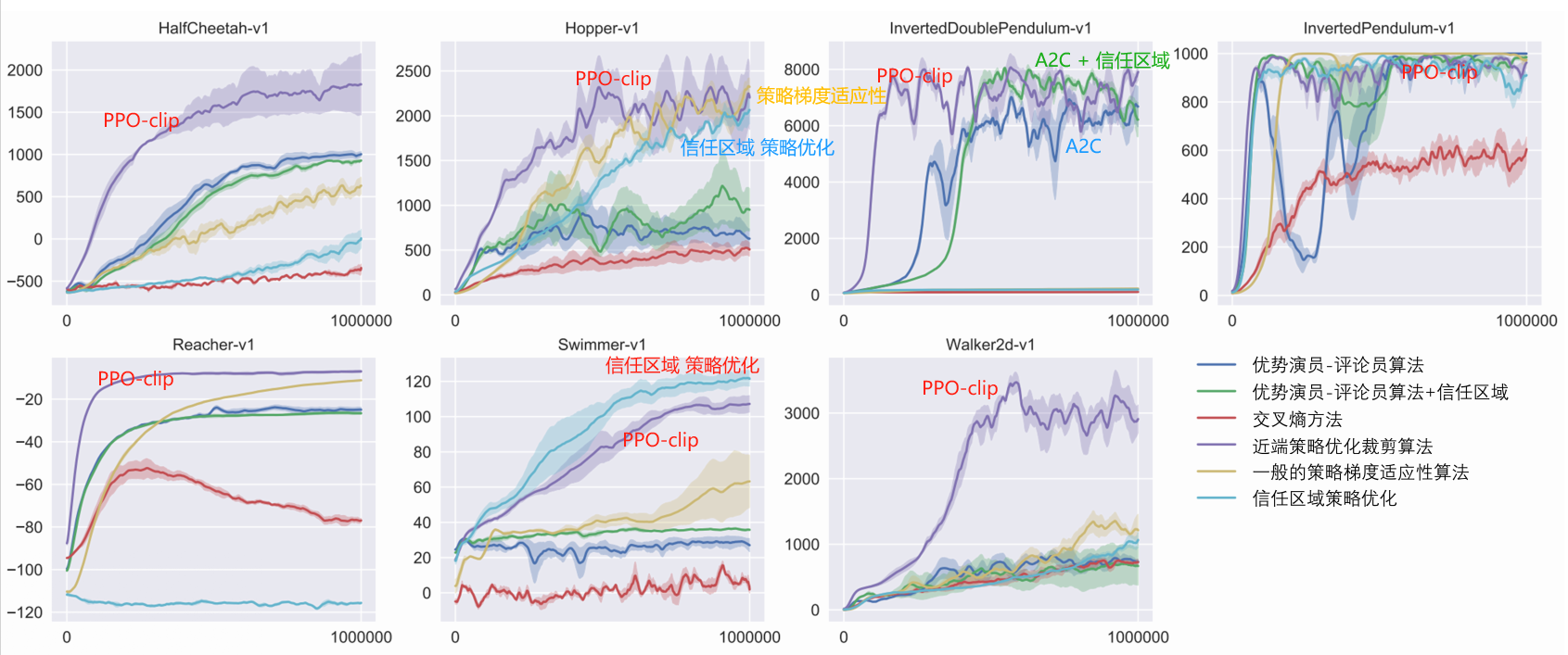
PPO

In practice, the clip constraint is generally used because it is simpler, less computationally expensive, and produces better results.

The off-policy algorithm canTo use historical experience, generally use experience replay to store and reuse previous experience,High data utilization efficiency。

PPO is an on-policy algorithm

• Although the importance sampling part uses the old actor sampling samples, weWe do not use these samples directly to update the strategy., but use importance sampling to correct the error caused by different data distributions, that is, to minimize the difference between the two sample distributions. In other words, it can be understood that although the samples after importance sampling are obtained by sampling with the old strategy,is approximately obtained from the updated policy, that is, the actor we want to optimize and the actor sampled are the same.

——————————————————

— OpenAI Documentation_PPO

OpenAI Documentation
Paper arXiv interface link: Proximal Policy Optimization Algorithms

PPO: on-policy algorithm, applicable to discrete or continuous action space. Possible local optimum

The motivation for PPO is the same as TRPO: how to use existing dataTake the biggest possible step in strategy improvement, without changing it too much and accidentally causing performance problems?
TRPO tries to solve this problem with a complicated second-order method, while PPO is a first-order method that uses some other tricks to keep the new policy close to the old one.
The PPO method is much simpler to implement and has been empirically shown to perform at least as well as TRPO.

There are two main variations of PPO: PPO-Penalty and PPO-Clip.

• PPO-Penalty approximately solves the KL-constrained update like TRPO, but penalizes KL-divergence in the objective function instead of making it a hard constraint, and automatically adjusts the penalty coefficient during training so that it scales appropriately.
• PPO-Clip has no KL-divergence or constraints in the objective function. Instead, it relies on specific clipping of the objective function to remove the incentive for the new policy to move away from the old policy.
  PPO-Clip (the main variant used by OpenAl).

PPO-Clip algorithm pseudocode

Algorithm: PPO-Clip
1: Input: Initial strategy parameters${\theta }_0$, initial value function parameters ${\varphi }_0$
2：$\mathbf{for}k=0,1,2,\dots \mathbf{do}$：
3：        ~~~~~~       By running the policy in the environment ${\pi }_k=\pi ({\theta }_k)$ Collecting Trajectory Sets D k = { τ i } {cal D}_k={tau_i} Dk​={τi​}
4：        ~~~~~~       Calculating rewards (rewards-to-go) ${\hat{R}}_t$ ▢ ${\hat{R}}_t$ Calculation rules
5：        ~~~~~~       Compute advantage estimate, based on current value function $V_{{\varphi }_k}$ of${\hat{A}}_t$ (Use any dominance estimation method)       ~~~~~       ▢ What are the current methods for edge estimation?
6：        ~~~~~~       Update the policy by maximizing the PPO-Clip objective function:
            ~~~~~~~~~~~            
${\theta }_{k+1}=\arg \underset{\theta }{\max }\frac{1}{|{\mathcal{D}}_k|T}\sum _{\tau \in {\mathcal{D}}_k}\sum _{t=0}^T\min (\frac{{\pi }_{\theta }(a_t|s_t)}{{\pi }_{{\theta }_k}(a_t|s_t)}{A}^{{\pi }_{{\theta }_k}}(s_t,a_t),g(ϵ,A^{{\pi }_{{\theta }_k}}(s_t,a_t)))$       ~~~~~       ▢ How to determine the policy update formula?
            ~~~~~~~~~~~            
            ~~~~~~~~~~~             ${\pi }_{{\theta }_k}$: Policy parameter vector before update. Importance sampling. Sampling from the old policy.
            ~~~~~~~~~~~            
            ~~~~~~~~~~~            General Stochastic Gradient Ascent + Adam
7：        ~~~~~~       Mean square errorRegression fit value function:
            ~~~~~~~~~~~            
${\varphi }_{k+1}=\arg \underset{\varphi }{\min }\frac{1}{|{\mathcal{D}}_k|T}\sum _{\tau \in {\mathcal{D}}_k}\sum _{t=0}^T(V_{\varphi }(s_t)-{\hat{R}}_t{)}^2$
            ~~~~~~~~~~~            
            ~~~~~~~~~~~            General Gradient Descent
8：$\mathbf{end}\mathbf{for}$
             ~~~~~~~~~~~~             

$dots$$\dots$

$g(ϵ,A)=\{\begin{array}{rlr}& (1+ϵ)A& A\ge 0\\ & (1-ϵ)A& A<0\end{array}$

In the paperAdvantage Estimate:

${\hat{A}}_t=-V(s_t)+\underset{{\hat{R}}_t???}{\underbrace{r_t+\gamma r_{t+1}+\cdots +{\gamma }^{T-t+1}{r}_{T-1}+{\gamma }^{T-t}V(s_T)}}$

make ${\Delta }_t=r_t+\gamma V(s_{t+1})-V(s_t)$
but$r_t={\Delta }_t-\gamma V(s_{t+1})+V(s_t)$

Substitution ${\hat{A}}_t$ expression

$\begin{array}{rl}{\hat{A}}_t& =-V(s_t)+r_t+\gamma r_{t+1}+{\gamma }^2{r}_{t+2}+\cdots +{\gamma }^{T-t}{r}_{T-2}+{\gamma }^{T-t+1}{r}_{T-1}+{\gamma }^{T-t}V(s_T)\\ & =-V(s_t)+r_t+\gamma r_{t+1}+\cdots +{\gamma }^{T-t+1}{r}_{T-1}+{\gamma }^{T-t}V(s_T)\\ & =-V(s_t)+\\ & {\Delta }_t-\gamma V(s_{t+1})+V(s_t)+\\ & \gamma ({\Delta }_{t+1}-\gamma V(s_{t+2})+V(s_{t+1}))+\\ & {\gamma }^2({\Delta }_{t+2}-\gamma V(s_{t+3})+V(s_{t+1}))+\\ & \cdots +\\ & {\gamma }^{T-t}({\Delta }_{T-t}-\gamma V(s_{T-t+1})+V(s_{T-t}))+\\ & {\gamma }^{T-t+1}({\Delta }_{T-1}-\gamma V(s_T)+V(s_{T-1}))+\\ & {\gamma }^{T-t}V(s_T)\\ & ={\Delta }_t+\gamma {\Delta }_{t+1}+{\gamma }^2{\Delta }_{t+2}+\cdots +{\gamma }^{T-t}{\Delta }_{T-t}+{\gamma }^{T-t+1}{\Delta }_{T-1}\end{array}$

Clipping acts as a regularizer by removing the incentive to make drastic policy changes.Hyperparameters $ϵ$ Corresponding to the distance between the new strategy and the old strategy。

This kind of clipping may still end up with a new strategy that is far from the old one. In the implementation here, we use a particularly simple method:Early StoppingIf the average KL-divergence between the new policy and the old policy exceeds a threshold, we stop executing the gradient step.

Simple derivation of PPO objective function link
The objective function of PPO-Clip is:
  ~  
$L_{{\theta }_k}^{\mathrm{CLIP}}(\theta )=\underset{s,a\sim {\theta }_k}{E}\left[\min \right(\frac{{\pi }_{\theta }(a|s)}{{\pi }_{{\theta }_k}(a|s)}{A}^{{\theta }_k}(s,a),\mathrm{clip}(\frac{{\pi }_{\theta }(a|s)}{{\pi }_{{\theta }_k}(a|s)},1-ϵ,1+ϵ)A^{{\theta }_k}(s,a)\left)\right]$
  ~  
$underset{s, asimtheta_k}{rm E}$$\underset{s,a\sim {\theta }_k}{E}$
  ~  
No.$k$ The strategy parameters for the iteration${\theta }_k$， $ϵ$ is a small hyperparameter.
set up$ϵ\in (0,1)$, Definition
$F(r,A,ϵ)\doteq \min (rA,\mathrm{clip}(r,1-ϵ,1+ϵ)A)$
when $A\ge 0$
$\begin{array}{rl}F(r,A,ϵ)& =\min (rA,\mathrm{clip}(r,1-ϵ,1+ϵ)A)\\ & =A\min (r,\mathrm{clip}(r,1-ϵ,1+ϵ))\\ & =A\min (r,\left\{\begin{array}{rlr}& 1+ϵ& r\ge 1+ϵ\\ & r& r\in (1-ϵ,1+ϵ)\\ & 1-ϵ& r\le 1-ϵ\end{array}\right\})\\ & =A\left\{\begin{array}{rlr}& \min (r,1+ϵ)& r\ge 1+ϵ\\ & \min (r,r)& r\in (1-ϵ,1+ϵ)\\ & \min (r,1-ϵ)& r\le 1-ϵ\end{array}\right\}\\ & =A\left\{\begin{array}{rlr}& 1+ϵ& r\ge 1+ϵ\\ & r& r\in (1-ϵ,1+ϵ)\\ & r& r\le 1-ϵ\end{array}\right\}According\; to\; the\; range\; on\; the\; right\\ & =A\min (r,1+ϵ)\\ & =\min (rA,(1+ϵ)A)\end{array}$
  ~  
when $A<0$
$\begin{array}{rl}F(r,A,ϵ)& =\min (rA,\mathrm{clip}(r,1-ϵ,1+ϵ)A)\\ & =A\max (r,\mathrm{clip}(r,1-ϵ,1+ϵ))\\ & =A\max (r,\left\{\begin{array}{rlr}& 1+ϵ& r\ge 1+ϵ\\ & r& r\in (1-ϵ,1+ϵ)\\ & 1-ϵ& r\le 1-ϵ\end{array}\right\})\\ & =A\left\{\begin{array}{rlr}& \max (r,1+ϵ)& r\ge 1+ϵ\\ & \max (r,r)& r\in (1-ϵ,1+ϵ)\\ & \max (r,1-ϵ)& r\le 1-ϵ\end{array}\right\}\\ & =A\left\{\begin{array}{rlr}& r& r\ge 1+ϵ\\ & r& r\in (1-ϵ,1+ϵ)\\ & 1-ϵ& r\le 1-ϵ\end{array}\right\}According\; to\; the\; range\; on\; the\; right\\ & =A\max (r,1-ϵ)\\ & =\min (rA,(1-ϵ)A)\end{array}$
  ~  
In summary: it can be defined$g(ϵ,A)$
$g(ϵ,A)=\{\begin{array}{rlr}& (1+ϵ)A& A\ge 0\\ & (1-ϵ)A& A<0\end{array}$

Why does this definition ensure that the new strategy does not stray too far from the old one?
Importance sampling methods effectively require new strategies ${\pi }_{\theta }(a|s)$ and the old strategy${\pi }_{{\theta }_k}(a|s)$ The two distributions cannot be too far apart

1. When advantage is positive

$L(s,a,{\theta }_k,\theta )=\min (\frac{{\pi }_{\theta }(a|s)}{{\pi }_{{\theta }_k}(a|s)},1+ϵ)A^{{\pi }_{{\theta }_k}}(s,a)$
Advantage function: If a state-action pair is found to have a high reward, increase the weight of the state-action pair.

When the state-action pair $(s,a)$ The advantage of is positive, then if the action$a$ is more likely to be executed if${\pi }_{\theta }(a|s)$ Increase, and the goal will increase.
The min in this item limits the objective function to only increase to a certain value
once${\pi }_{\theta }(a|s)>(1+ϵ){\pi }_{{\theta }_k}(a|s)$, min trigger, limit the value of this item $(1+ϵ){\pi }_{{\theta }_k}(a|s)$。
the new policy does not benefit by going far away from the old policy.
New strategies do not benefit from moving away from old strategies.

2. When the advantage is negative

$L(s,a,{\theta }_k,\theta )=\max (\frac{{\pi }_{\theta }(a|s)}{{\pi }_{{\theta }_k}(a|s)},1-ϵ)A^{{\pi }_{{\theta }_k}}(s,a)$

When a state-action pair $(s,a)$ The advantage of is negative, then if the action is executed$a$ is less likely, that is, if${\pi }_{\theta }(a|s)$ If decreases, the objective function will increase. However, the max in this term limits how much the objective function can increase.
once${\pi }_{\theta }(a|s)<(1-ϵ){\pi }_{{\theta }_k}(a|s)$, max trigger, limit the value of this item to $(1-ϵ){\pi }_{{\theta }_k}(a|s)$。

To reiterate: the new policy does not benefit by going far away from the old policy.
New strategies do not benefit from moving away from old strategies.

TD3_Continuous only： Twin Delayed Deep Deterministic Policy Gradient [ICML 2018 (Canada) McGill University]

Image Source

OpenAI Documentation_TD3
Paper link

While DDPG can sometimes achieve excellent performance, it is often unstable when it comes to hyperparameters and other types of tuning.
A common DDPG failure mode is that the learned Q-function starts to significantly overestimate the Q-values, which then causes the policy to break because it exploits the error in the Q-function.
Twin Delayed DDPG (TD3) is an algorithm that solves this problem by introducing three key tricks:
1、Truncated Double Q Learning。

• TD3 learns two Q-functions instead of one (hence "twin"), and uses the smaller of the two Q-values ​​to form the target in the Bellman error loss function.

2、Policy update delay。

• TD3 updates the policy (and target network) less frequently than the Q function. The paper suggests updating the policy once for every two updates of the Q function.

3. Target strategy smoothing.

• TD3 adds noise to the target action, making it harder for the policy to exploit the error in the Q function by smoothing out the changes in the action.

TD3 is an off-policy algorithm; it can only be used withcontinuousThe environment of the action space.

TD3 algorithm pseudocode

Algorithm: TD3
With random parameters${\theta }_1,{\theta }_2,\varphi$ Initialize the critic network$Q_{{\theta }_1},Q_{{\theta }_2}$, and actor networks ${\pi }_{\varphi }$
Initialize the target network${\theta }_1^{\prime }\leftarrow {\theta }_1,{\theta }_2^{\prime }\leftarrow {\theta }_2,{\varphi }^{\prime }\leftarrow \varphi$
Initialize the playback buffer set$\mathcal{B}$
$\mathbf{for}t=1\mathbf{to}T$ ：
       ~~~~~~       Selecting actions with exploration noise $a\sim {\pi }_{\varphi }(s)+ϵ,ϵ\sim \mathcal{N}(0,\sigma )$, Observation Reward $r$ and the new state$s^{\prime }$
       ~~~~~~       The transition tuple $(s,a,r,s^{\prime })$ Save to$\mathcal{B}$ middle
       ~~~~~~       from $\mathcal{B}$ Sampling small batches$N$ transitions$(s,a,r,s^{\prime })$
$\tilde{a}\leftarrow {\pi }_{{\varphi }^{\prime }}(s^{\prime })+ϵ,ϵ\sim \mathrm{clip}(\mathcal{N}(0,\tilde{\sigma }),-c,c)$
$y\leftarrow r+\gamma \underset{i=1,2}{\min }{Q}_{{\theta }_i^{\prime }}(s^{\prime },\tilde{a})$
       ~~~~~~       Update critics ${\theta }_i\leftarrow \arg \underset{{\theta }_i}{\min }{N}^{-1}\sum (y-Q_{{\theta }_i}(s,a){)}^2$
       ~~~~~~        $\mathbf{if}t\%d$：
            ~~~~~~~~~~~            Updated via deterministic policy gradient $\varphi$
${\nabla }_{\varphi }J(\varphi )=N^{-1}\sum {\nabla }_a{Q}_{{\theta }_1}(s,a){|}_{a={\pi }_{\varphi }(s)}{\nabla }_{\varphi }{\pi }_{\varphi }(s)$
            ~~~~~~~~~~~            Update the target network:
${\theta }_i^{\prime }\leftarrow \tau {\theta }_i+(1-\tau ){\theta }_i^{\prime }$$\tau$: Target update rate
${\varphi }^{\prime }\leftarrow \tau \varphi +(1-\tau ){\varphi }^{\prime }$
$\mathbf{end}\mathbf{if}$
$\mathbf{end}\mathbf{for}$

Soft Actor-Critic: SAC_Continuous/Discrete Action Space [Google Brain latest version 201906]

Image Source

Maximize the entropy of the policy, thus making the policy more robust.

Deterministic Strategy It means that given the same state, the same action is always chosen.
Randomness strategy There are multiple possible actions that can be chosen in a given state.

In practical applications, if conditions permit, we willUse as much as possibleRandomness strategy, such as A2C, PPO, etc., because it is more flexible, more robust and more stable.

Maximum entropy reinforcement learning believes that even though we currently have mature random strategies, such as AC algorithms, we still have not achieved optimal randomness. Therefore, it introduces aInformation EntropyThe concept ofMaximize the cumulative reward while maximizing the entropy of the strategy, making the strategy more robust, thus achieving the optimal stochastic strategy.

——————————————————

— OpenAI Documentation_SAC

OpenAI Documentation_SAC interface link
  ~  
Soft Actor-Critic: Off-Policy Maximum Entropy Deep Reinforcement Learning with a Stochastic Actor, Haarnoja et al, 201808 ICML 2018
Soft Actor-Critic Algorithms and Applications, Haarnoja et al, 201901
Learning to Walk via Deep Reinforcement Learning, Haarnoja et al, 201906 RSS2019

Soft Actor Critic (SAC) optimizes random policies in an off-policy manner.

DDPG + Stochastic Strategy Optimization

Not a direct successor to TD3 (published almost simultaneously).

It incorporates the clipped double-Q trick, and due to the inherent randomness of SAC's strategy, it also ultimately benefits fromTarget strategy smoothing。

A core feature of SAC is entropy regularization。
The policy is trained to maximize the trade-off between expected reward and entropy,Entropy is a measure of the randomness of a policy。
This is closely related to the trade-off between exploration and exploitation: an increase in entropy leads toMore to explore,this is OKAccelerate subsequent learningIt can alsoPrevent the strategy from converging to a bad local optimum prematurely。

It can be used in both continuous and discrete action spaces.

exist Entropy-Regularized Reinforcement LearningIn the example, the agent obtains the sameThe entropy of the policy at this time stepProportional rewards.
At this time, the RL problem is described as:

${\pi }^{\ast }=\arg \underset{\pi }{\max }\underset{\tau \sim \pi }{E}\left[\sum _{t=0}^{\infty }{\gamma }^t\right(R(s_t,a_t,s_{t+1})+\alpha H(\pi (\cdot |s_t)))]$

in $\alpha >0$ is the trade-off coefficient.
The state-value function includes an entropy bonus at each time step$V^{\pi }$ for:

$V^{\pi }(s)=\underset{\tau \sim \pi }{E}\left[\sum _{t=0}^{\infty }{\gamma }^t\right(R(s_t,a_t,s_{t+1})+\alpha H(\pi (\cdot |s_t)))|s_0=s]$

Action-value function including entropy bonus for every time step except the first $Q^{\pi }$:

$Q^{\pi }(s,a)=\underset{\tau \sim \pi }{E}\left[\sum _{t=0}^{\infty }{\gamma }^t\right(R(s_t,a_t,s_{t+1})+\alpha \sum _{t=1}^{\infty }H(\pi (\cdot |s_t)))|s_0=s,a_0=a]$

• Some papers $Q^{\pi }$ Contains the entropy reward for the first time step

$V^{\pi }$ and$Q^{\pi }$ The relationship between them is:

$V^{\pi }(s)=\underset{a\sim \pi }{E}[Q^{\pi }(s,a)]+\alpha H(\pi (\cdot |s))$

about $Q^{\pi }$ The Bellman formula is:

$\begin{array}{rl}{Q}^{\pi }(s,a)& =\underset{\genfrac{}{}{0ex}{}{s^{\prime }\sim P}{a^{\prime }\sim \pi }}{E}[R(s,a,s^{\prime })+\gamma (Q^{\pi }(s^{\prime },a^{\prime })+\alpha H(\pi (\cdot |s^{\prime })))]\\ & =\underset{s^{\prime }\sim P}{E}[R(s,a,s^{\prime })+\gamma V^{\pi }(s^{\prime })]\end{array}$

SAC learns a policy at the same time ${\pi }_{\theta }$ and two$Q$ function$Q_{{\varphi }_1},Q_{{\varphi }_2}$。
There are currently two standard SAC variants: one that uses a fixedEntropy regularization coefficient $\alpha$, and another by changing $\alpha$ to enforce the entropy constraint.
OpenAI's documentation uses a version with a fixed entropy regularization coefficient, but in practice one usually prefersEntropy ConstraintVariant of .

As shown in the figure below, $\alpha$ In the fixed version, except for the last figure which has a clear advantage, the others are only slightly better, basically the same as$\alpha$ The learning version is flat;$\alpha$ The learning version has advantages in the two middle pictures, with more obvious advantages.

Image Source

SAC VS TD3:
  ~  
Same point:
1. Both Q functions are learned by regressing to a single shared objective by minimizing the MSBE (Mean Squared Bellman Error).
2. Use the target Q-network to calculate the shared target, and perform polyak averaging on the Q-network parameters during training to obtain the target Q-network.
3. The shared target uses a truncated double Q technique.
  ~  
difference:
1. SAC contains entropy regularization term
2. The next state action used in SAC’s goal comes fromCurrent Strategy, rather than a target strategy.
3. There is no clear target policy smoothing. TD3 trains a deterministic policy that takes actions to the next state.Add random noiseSAC trains a random policy, and the noise from randomness is enough to achieve similar effects.

SAC algorithm pseudocode

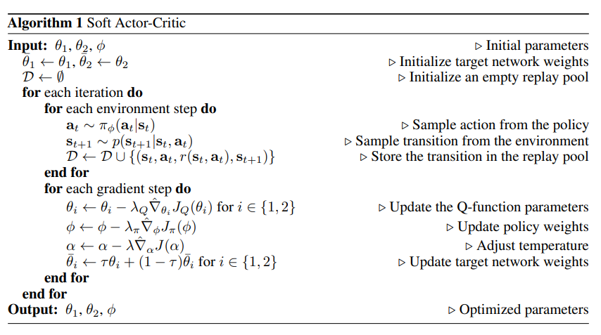
Algorithm: Soft Actor-Critic SAC
enter:${\theta }_1,{\theta }_2,\varphi$ Initialization parameters
Parameter initialization:
       ~~~~~~       Initialize the target network weights:${\bar{\theta }}_1\leftarrow {\theta }_1,{\bar{\theta }}_2\leftarrow {\theta }_2$
       ~~~~~~       The playback pool is initialized to be empty:$\mathcal{D}\leftarrow \varnothing$
$\mathbf{for}$ Each iteration$\mathbf{do}$ ：
       ~~~~~~       $\mathbf{for}$ Each environment step$\mathbf{do}$ ：
            ~~~~~~~~~~~            Sample actions from the policy: $a_t\sim {\pi }_{\varphi }(a_t|s_t)$ ▢ Here ${\pi }_{\varphi }(a_t|s_t)$ How to define?
            ~~~~~~~~~~~            Sample transitions from the environment:$s_{t+1}\sim p(s_{t+1}|s_t,a_t)$
            ~~~~~~~~~~~            Save the transition to the replay pool: $\mathcal{D}\leftarrow \mathcal{D}\cup \{(s_t,a_t,r(s_t,a_t),s_{t+1})\}$
       ~~~~~~       $\mathbf{end}\mathbf{for}$
       ~~~~~~       $\mathbf{for}$ Each gradient step$\mathbf{do}$ ：
            ~~~~~~~~~~~            renew $Q$ Function parameters: For i ∈ { 1 , 2 } iin{1,2} i∈{1,2}，${\theta }_i\leftarrow {\theta }_i-{\lambda }_Q{\hat{\nabla }}_{{\theta }_i}{J}_Q({\theta }_i)$ ▢ Here $J_Q({\theta }_i)$ How to define?
            ~~~~~~~~~~~            Update policy weights: $\varphi \leftarrow \varphi -{\lambda }_{\pi }{\hat{\nabla }}_{\varphi }{J}_{\pi }(\varphi )$ ▢ Here $J_{\pi }(\varphi )$ How to define?
            ~~~~~~~~~~~            Adjust the temperature: $\alpha \leftarrow \alpha -\lambda {\hat{\nabla }}_{\alpha }J(\alpha )$ ▢ Here $J(\alpha )$ How to define? How to understand the temperature here
            ~~~~~~~~~~~             Update the target network weights: For i ∈ { 1 , 2 } iin{1,2} i∈{1,2}，${\bar{\theta }}_i\leftarrow \tau {\theta }_i-(1-\tau ){\bar{\theta }}_i$ ▢ How to understand this $\tau$? ——&gt; Target smoothing coefficient
       ~~~~~~       $\mathbf{end}\mathbf{for}$
$\mathbf{end}\mathbf{for}$
Output:${\theta }_1,{\theta }_1,\varphi$Optimized parameters

$\hat{\nabla }$： Stochastic gradient

$emptyset$$\varnothing$

Learning to Walk via Deep Reinforcement Learning Versions in:
  ~  

$\alpha$ is the temperature parameter, which determines the relative importance of the entropy term and the reward, thereby controlling the stochasticity of the optimal policy.
$\alpha$ Large: Explore
$\alpha$ Small: Utilize

$J(\alpha )=\underset{a_t\sim {\pi }_t}{\mathbb{E}}[-\alpha \log {\pi }_t(a_t|s_t)-\alpha \bar{\mathcal{H}}]$