Technology Sharing

한어Русский языкEnglishFrançaisIndonesianSanskrit日本語DeutschPortuguêsΕλληνικάespañolItalianoSuomalainenLatina

Table of contents

Beyond a single randomized controlled trial

Aggregating difference-in-means estimators

Continuous X and the propensity score

---

One of the simplest extensions of randomized trials is the estimation of intervention effects under no constraints. Qualitatively, unboundedness is relevant when we want to estimate a treatment effect that is not random but is as good as if it were random once we control for a set of covariates Xi.

The purpose of this lecture is to discuss the identification and estimation of average intervention effects under this unbounded assumption. As before, we will adopt a nonparametric approach: we will not assume any good specification of the parametric model, and the identification of the average treatment effect will be driven entirely by the design (i.e., conditional independence statements associated with the potential intervention outcome and the treatment).

Beyond a single randomized controlled trial

We define the causal effect of a treatment in terms of potential intervention outcomes. For a binary intervention w∈{0, 1}, we define potential outcomes Yi(1) and Yi(0) corresponding to the outcomes that the ith subject would experience if he or she received or did not receive the intervention, respectively. We assume SUTVA,, and wish to estimate the average intervention effect

In the first lecture, we assumed random intervention assignment., and several √n-consistency estimators of ATE are studied.

The simplest way to go beyond one RCT is to think of two RCTs. To take a concrete example, suppose we are interested in giving adolescents cash incentives to stop them from smoking. 5% of adolescents in Palo Alto, California, and 20% of adolescents in Geneva, Switzerland, are eligible to participate in this study.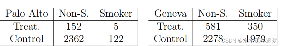

Within each city, we did a randomized controlled study and it was easy to see that the intervention helped. However, looking at the aggregate data was misleading and made it look like the intervention hurt; this is an example of what is sometimes called Simpson's paradox: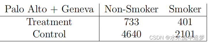Once we pool the data, this is no longer an RCT, as people in Geneva are both more likely to receive treatment and more likely to smoke regardless of whether they receive treatment. To get a consistent estimate of ATE, we need to estimate the intervention effect in each city separately:

What are the statistical properties of this estimator? How does this idea generalize to continuous x?

Aggregating difference-in-means estimators

Assume that the covariate Xi takes values ​​in the discrete space Xi∈X,. Assume again that treatment assignment is random assignment conditional on Xi (ie, each group has an RCT defined by the x levels):

The average treatment effect within the group is defined as

We can then estimate ATE τ by aggregating the group-level treatment effect estimates, as described above,

in ，How good is this estimate? Intuitively, we need to estimate "parameters", so we might expect the variance to be linear in p?

To explore this estimate, we can write it as follows. First, for any group with covariate x, define e(x) as the probability of being treated in that group, , and noted

In addition, according to Without relying on the simplifying assumptions about w, we can obtain

Next, for the ensemble estimator, defined as The proportion of observations will be Defined as its expected value, we can derive

Putting these parts together, we get

It is worth noting that the asymptotic variance VAGG does not depend on the number of groups. As we will see later, this fact plays a key role in making efficient semiparametric inferences about average intervention effects in observational studies.

Continuous X and the propensity score

Above, we considered the case where X is discrete with a finite number of levels, and the treatment Wi is random as in (2.1) with Xi = x. In this case, we found that we can still accurately estimate ATE by aggregating the within-group treatment effect estimates, and that the exact number of groups |X| = p does not affect the accuracy of the inference. However, if X is continuous (or the chi-square of X is very large), this result does not apply directly - since we cannot obtain enough samples for every possible value of x∈X to define τ(x) as in (2.3).

To generalize our analysis beyond the discrete-X case, we can no longer simply try to estimate τ(x) for each value of x by simple averaging, but instead use a more indirect argument. To do this, we first need to generalize the assumption that there is an RCT for each group. Formally, we simply write the same

Although Xi may now be an arbitrary random variable, this statement may need to be interpreted more cautiously. From a qualitative perspective, one way to interpret (2.6) is that we have measured enough covariates to capture any dependencies between Wi and the potential outcomes, so that given Xi, Wi cannot "peek" at {Yi(0), Yi(1)}. We call this assumptionunconfoundedness.

Assumption (2.6) seems difficult to use in practice because it involves conditions on continuous random variables. However, as Rosenbaum and Rubin (1983) pointed out, by taking into account the propensity score

From a statistical point of view, a key property of the propensity score is that it is a balanced score: if (2.6) holds, then in practice

That is, we can actually eliminate the bias associated with non-random intervention assignment by controlling only e(X) instead of X. We can verify this claim by:

(2.8) means that if we can partition the observations into groups with (almost) constant values ​​of the propensity score e(x), then we can Variants of continuously estimate the average intervention effect.