2024-07-12
한어Русский языкEnglishFrançaisIndonesianSanskrit日本語DeutschPortuguêsΕλληνικάespañolItalianoSuomalainenLatina
Series articles directory and links
Previous:Machine Learning (V) -- Supervised Learning (5) -- Linear Regression 2
Next:Machine Learning (V) -- Supervised Learning (7) -- SVM1
tips:标题前有“***”的内容为补充内容,是给好奇心重的宝宝看的,可自行跳过。文章内容被“文章内容”删除线标记的,也可以自行跳过。“!!!”一般需要特别注意或者容易出错的地方。
本系列文章是作者边学习边总结的,内容有不对的地方还请多多指正,同时本系列文章会不断完善,每篇文章不定时会有修改。
由于作者时间不算富裕,有些内容的《算法实现》部分暂未完善,以后有时间再来补充。见谅!
文中为方便理解,会将接口在用到的时候才导入,实际中应在文件开始统一导入。
Logistic regression = linear regression + sigmoid function
Logistic Regression, in simple terms, is to find a straight line to divide a binary data set.
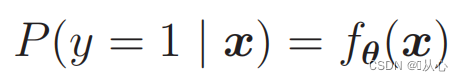
Solve the binary classification problem by belonging to a certain categoryProbability valueTo determine whether it belongs to a certain category, and this category is marked as 1 (positive example) by default, and the other category is marked as 0 (negative example).
In fact, this is similar to the linear regression steps. The difference lies in the different methods used for "checking the model fitting effect" and "adjusting the model position angle".
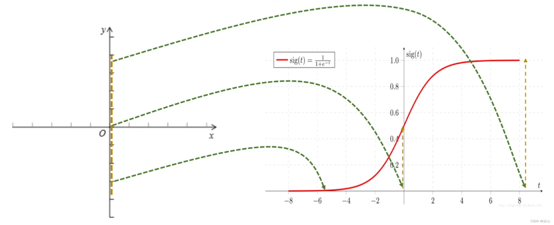
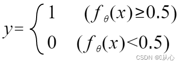
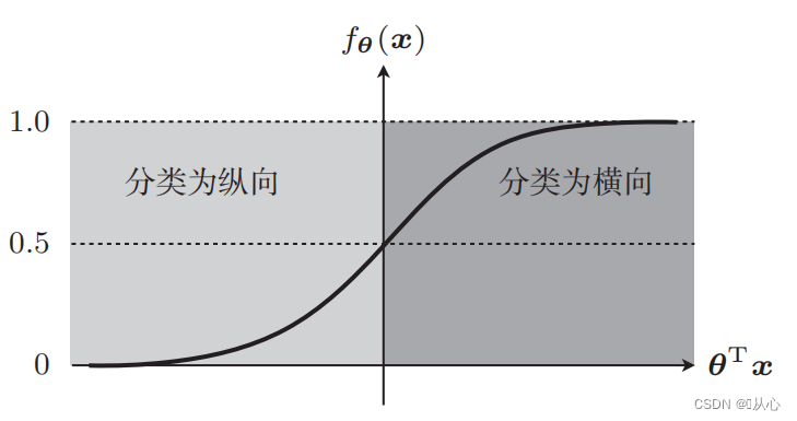
A function (sigmoid function) is needed to map the input data to between 0 and 1, and if the function value is greater than 0.5, it is judged to be 1, otherwise it is 0. In this way, it can be converted into a probability representation.
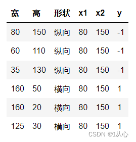
Taking picture classification as an example, the pictures are divided into vertical and horizontal
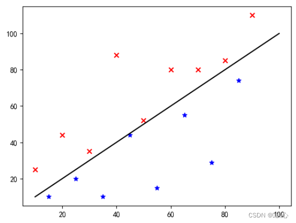
This is how we display these data on a graph. In order to separate the points of different colors (different categories) in the graph, we draw a line like this. The purpose of this classification is to find such a line.
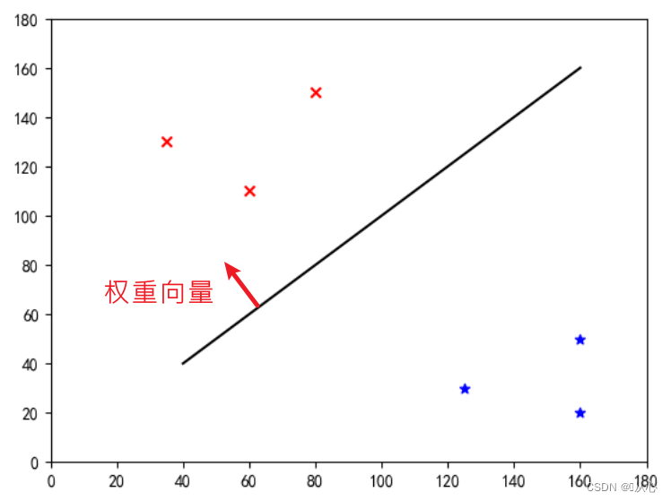
This is a line that "makes the weight vector the normal vector" (makes the weight vector perpendicular to the line)

w is the weight vector; make it a straight line of the normal vector, even if
A model that accepts multiple values, multiplies each value by its weight, and outputs the sum.
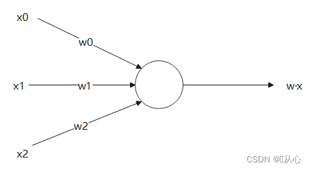
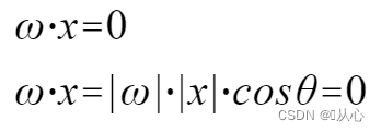
The inner product is an indicator to measure the similarity between vectors. A positive result indicates similarity, a 0 indicates verticality, and a negative result indicates dissimilarity.
use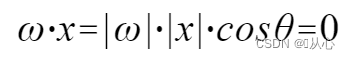 It is easier to understand because both |w| and |x| are positive numbers, so the sign of the inner product is determined by cosθ, that is, less than 90 degrees is similar, and greater than 90 degrees is dissimilar, that is,
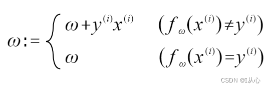
If the value is equal to the original label, the weight vector is not updated. If the value is not equal to the original label, the weight vector is updated by adding the vectors.
As shown in the figure, if it is not equal to the original label, then
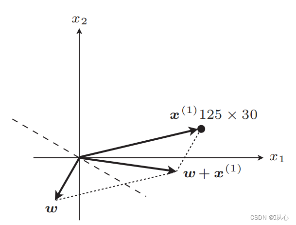
Updated straight line
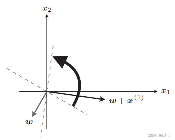
After updating, equal
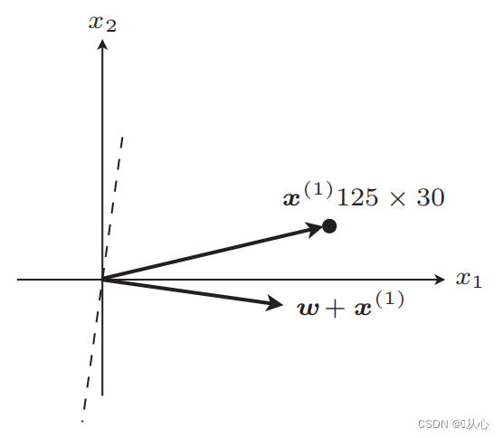
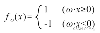
Steps: First randomly determine a straight line (that is, randomly determine a weight vector w), substitute the inner product into a real value data x, and get a value (1 or -1) through the discriminant function. If it is equal to the original label value, the weight vector is not updated. If it is not equal to the original label value, the weight vector is updated by adding the vectors.
!!! Note: Perceptron can only solve linearly separable problems
Linearly separable: situations where a straight line can be used for classification
Linearly inseparable: cannot be classified by a straight line
The black one is the sigmoid function, and the red one is the step function (discontinuous).
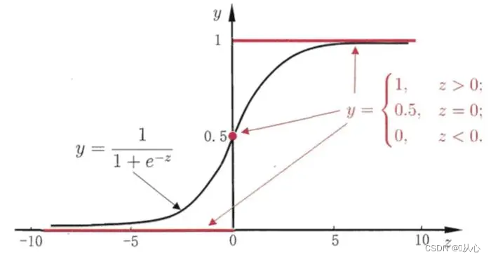
Function: The input of logistic regression is the result of linear regression.We can get a predicted value in linear regression. The Sigmoid function maps any input to the interval [0,1], thus completing the conversion from value to probability, which is the classification task.
Logistic regression = linear regression + sigmoid function
Linear Regression: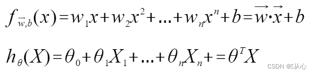
Sigmoid function: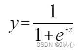
Logistic Regression: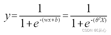
To make y represent the label, change it to:
To make probability use:
That is, the categories can be distinguished by probability
It can be rewritten as follows:
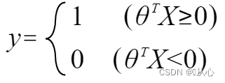
when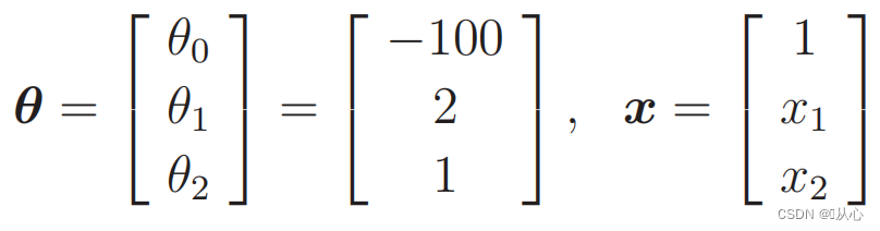
Substitute the data: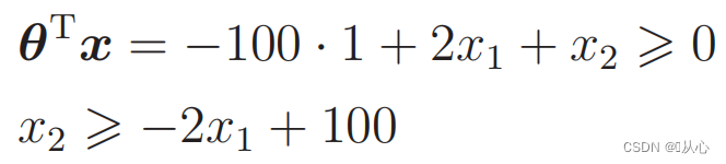
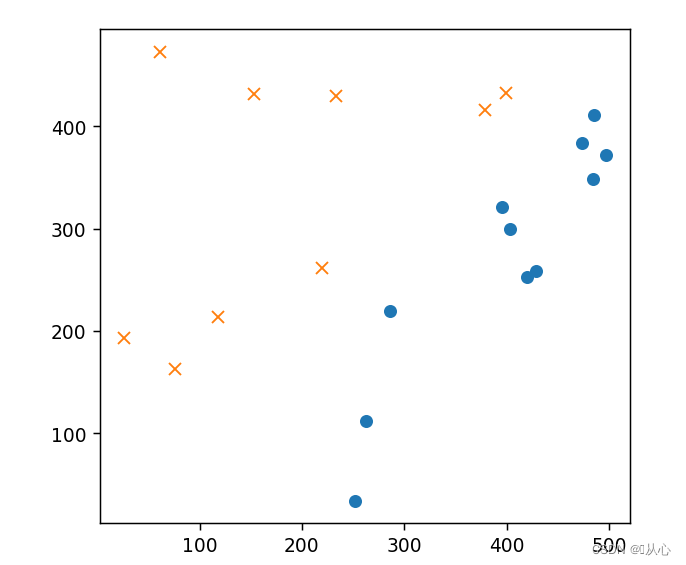
There is such a picture
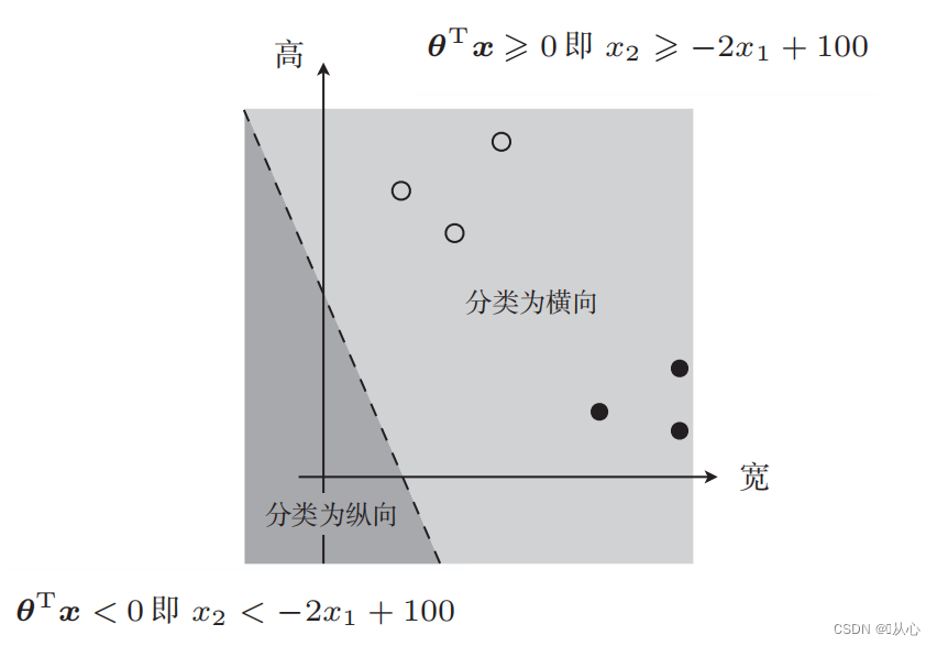 The straight line used to classify the data is the decision boundary.
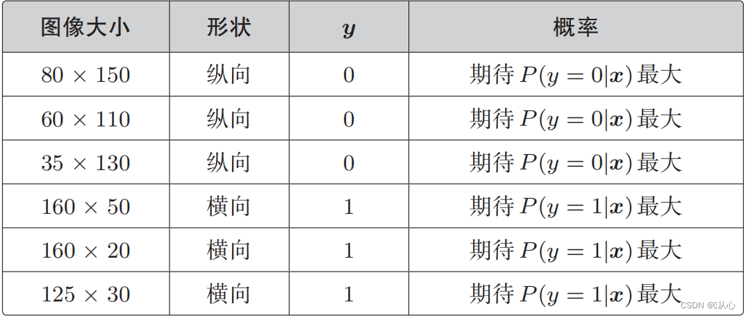
We hope that:
When y=1, P(y=1|x) is the largest
When y=0, P(y=0|x) is the largest
Likelihood function (joint probability): Here is the probability we want to maximize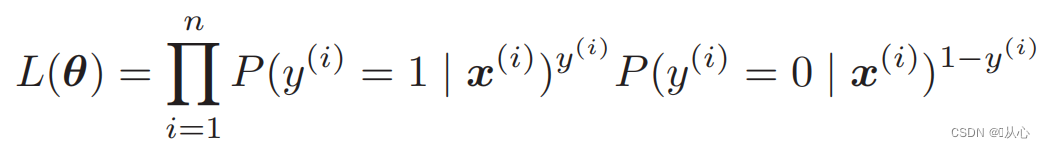
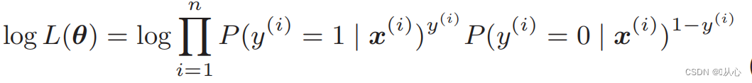
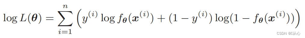
Log-likelihood function: It is difficult to differentiate the likelihood function directly, so we need to take the logarithm first.
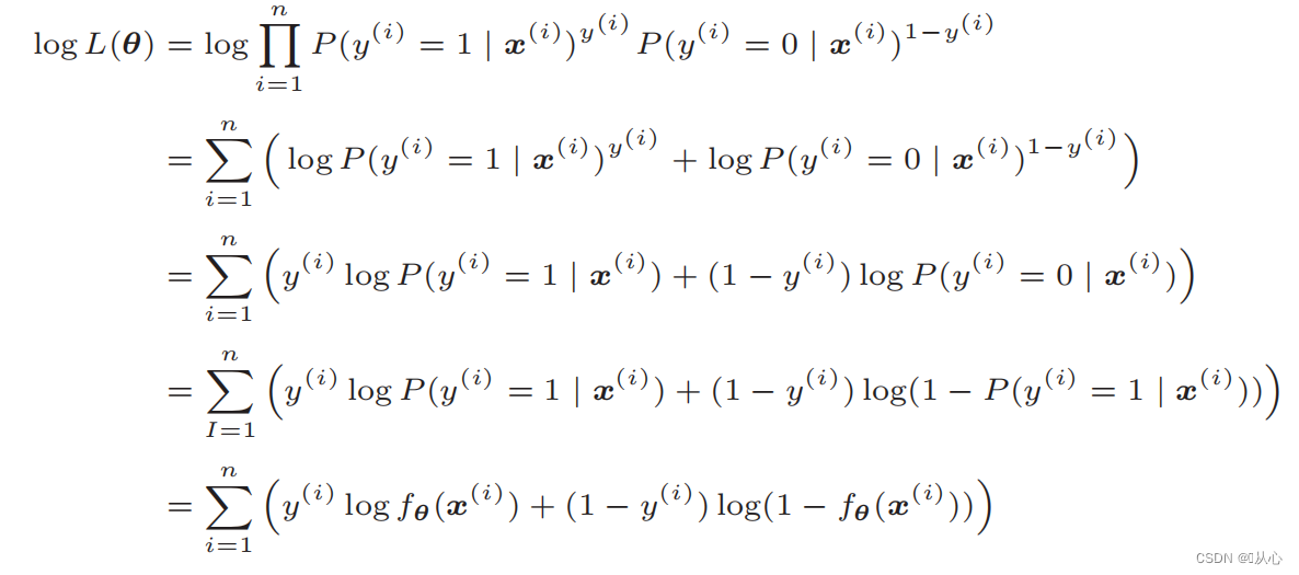
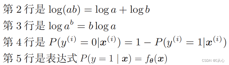
After deformation, it becomes:
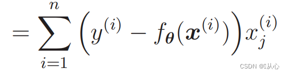
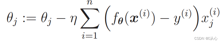
Differentiation of the likelihood function:

1. Simple implementation: Logistic regression is a simple algorithm that is easy to understand and implement.
2. High computational efficiency: Logistic regression requires relatively little computation and is suitable for large-scale data sets.
3. Strong interpretability: The output of logistic regression is a probability value, which can intuitively explain the output of the model.
1. Linear separability requirement: Logistic regression is a linear model and performs poorly for nonlinear separable problems.
2. Feature correlation problem: Logistic regression is sensitive to the correlation between input features. When there is a strong correlation between features, the performance of the model may deteriorate.
3. Overfitting problem: When there are too many sample features or the number of samples is small, logistic regression is prone to overfitting problems.
- import numpy as np
- import pandas as pd
- import matplotlib.pyplot as plt
- %matplotlib notebook
-
- # 读取数据
- train=pd.read_csv('csv/images2.csv')
- train_x=train.iloc[:,0:2]
- train_y=train.iloc[:,2]
- # print(train_x)
- # print(train_y)
-
- # 绘图
- plt.figure()
- plt.plot(train_x[train_y ==1].iloc[:,0],train_x[train_y ==1].iloc[:,1],'o')
- plt.plot(train_x[train_y == 0].iloc[:,0],train_x[train_y == 0].iloc[:,1],'x')
- plt.axis('scaled')
- # plt.axis([0,500,0,500])
- plt.show()
- # 初始化参数
- theta=np.random.randn(3)
-
- # 标准化
- mu = train_x.mean(axis=0)
- sigma = train_x.std(axis=0)
- # print(mu,sigma)
-
-
- def standardize(x):
- return (x - mu) / sigma
-
- train_z = standardize(train_x)
- # print(train_z)
-
- # 增加 x0
- def to_matrix(x):
- x0 = np.ones([x.shape[0], 1])
- return np.hstack([x0, x])
-
- X = to_matrix(train_z)
-
-
- # 绘图
- plt.figure()
- plt.plot(train_z[train_y ==1].iloc[:,0],train_z[train_y ==1].iloc[:,1],'o')
- plt.plot(train_z[train_y == 0].iloc[:,0],train_z[train_y == 0].iloc[:,1],'x')
- plt.axis('scaled')
- # plt.axis([0,500,0,500])
- plt.show()
- # sigmoid 函数
- def f(x):
- return 1 / (1 + np.exp(-np.dot(x, theta)))
-
- # 分类函数
- def classify(x):
- return (f(x) >= 0.5).astype(np.int)
- # 学习率
- ETA = 1e-3
-
- # 重复次数
- epoch = 5000
-
- # 更新次数
- count = 0
- print(f(X))
-
- # 重复学习
- for _ in range(epoch):
- theta = theta - ETA * np.dot(f(X) - train_y, X)
-
- # 日志输出
- count += 1
- print('第 {} 次 : theta = {}'.format(count, theta))
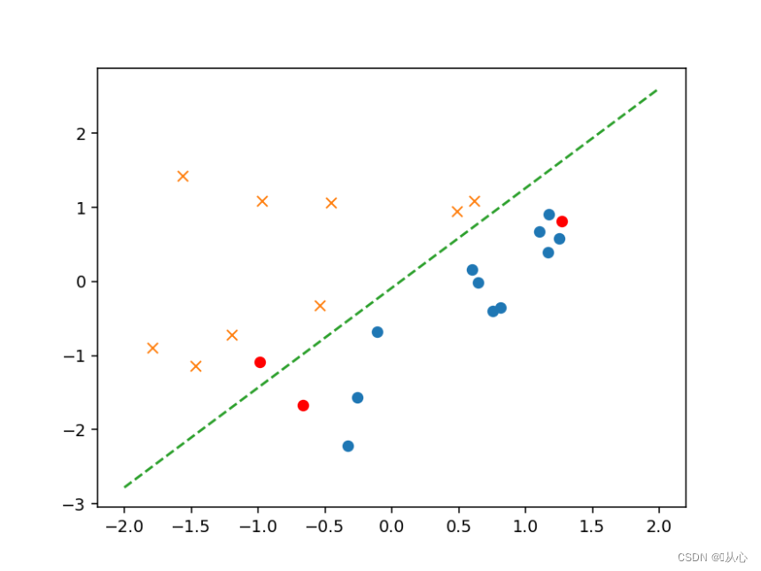
- # 绘图确认
- plt.figure()
- x0 = np.linspace(-2, 2, 100)
- plt.plot(train_z[train_y ==1].iloc[:,0],train_z[train_y ==1].iloc[:,1],'o')
- plt.plot(train_z[train_y == 0].iloc[:,0],train_z[train_y == 0].iloc[:,1],'x')
- plt.plot(x0, -(theta[0] + theta[1] * x0) / theta[2], linestyle='dashed')
- plt.show()
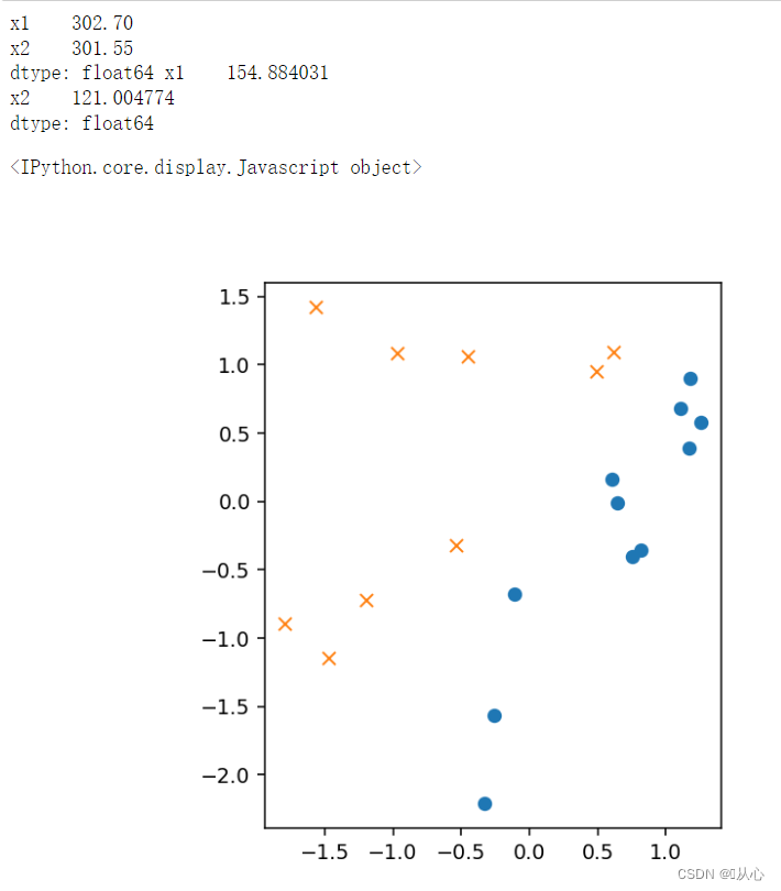
- # 验证
- text=[[200,100],[500,400],[150,170]]
- tt=pd.DataFrame(text,columns=['x1','x2'])
- # text=pd.DataFrame({'x1':[200,400,150],'x2':[100,50,170]})
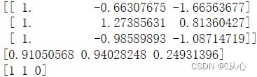
- x=to_matrix(standardize(tt))
- print(x)
- a=f(x)
- print(a)
-
- b=classify(x)
- print(b)
-
- plt.plot(x[:,1],x[:,2],'ro')
from sklearn.datasets import load_breast_cancer
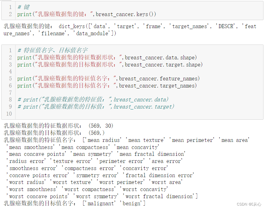
- # 键
- print("乳腺癌数据集的键:",breast_cancer.keys())
-
-
-
- # 特征值名字、目标值名字
- print("乳腺癌数据集的特征数据形状:",breast_cancer.data.shape)
- print("乳腺癌数据集的目标数据形状:",breast_cancer.target.shape)
-
- print("乳腺癌数据集的特征值名字:",breast_cancer.feature_names)
- print("乳腺癌数据集的目标值名字:",breast_cancer.target_names)
-
- # print("乳腺癌数据集的特征值:",breast_cancer.data)
- # print("乳腺癌数据集的目标值:",breast_cancer.target)
-
-
-
- # 返回值
- # print("乳腺癌数据集的返回值:n", breast_cancer)
- # 返回值类型是bunch--是一个字典类型
-
- # 描述
- # print("乳腺癌数据集的描述:",breast_cancer.DESCR)
-
-
-
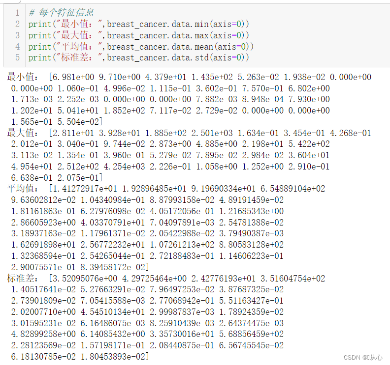
- # 每个特征信息
- print("最小值:",breast_cancer.data.min(axis=0))
- print("最大值:",breast_cancer.data.max(axis=0))
- print("平均值:",breast_cancer.data.mean(axis=0))
- print("标准差:",breast_cancer.data.std(axis=0))
-
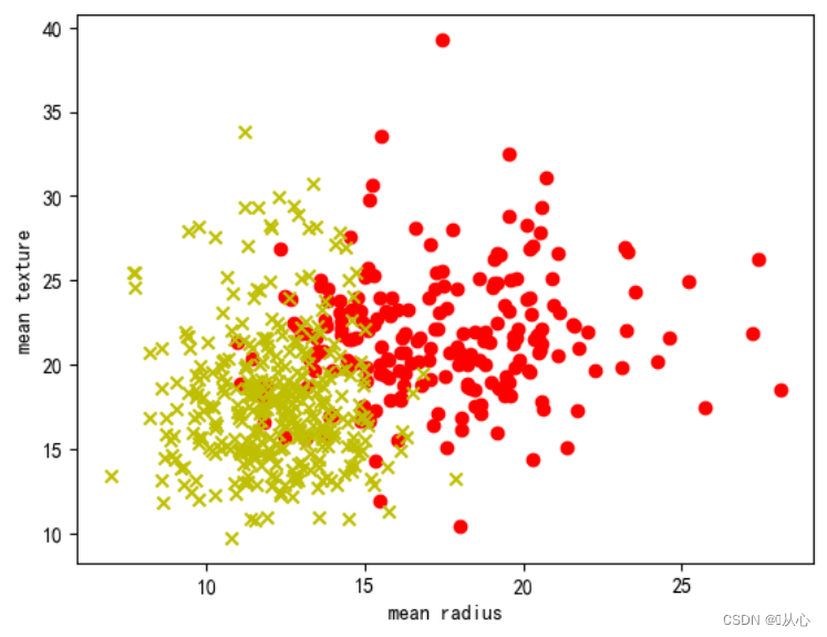
- # 取其中间两列特征
- x=breast_cancer.data[0:569,0:2]
- y=breast_cancer.target[0:569]
-
- samples_0 = x[y==0, :]
- samples_1 = x[y==1, :]
-
-
-
- # 实现可视化
- plt.figure()
- plt.scatter(samples_0[:,0],samples_0[:,1],marker='o',color='r')
- plt.scatter(samples_1[:,0],samples_1[:,1],marker='x',color='y')
- plt.xlabel('mean radius')
- plt.ylabel('mean texture')
- plt.show()
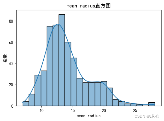
- # 绘制每个特征直方图,显示特征值的分布情况。
- for i, feature_name in enumerate(breast_cancer.feature_names):
- plt.figure(figsize=(6, 4))
- sns.histplot(breast_cancer.data[:, i], kde=True)
- plt.xlabel(feature_name)
- plt.ylabel("数量")
- plt.title("{}直方图".format(feature_name))
- plt.show()
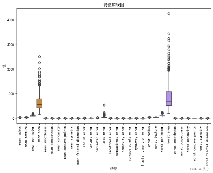
- # 绘制箱线图,展示每个特征最小值、第一四分位数、中位数、第三四分位数和最大值概括。
- plt.figure(figsize=(10, 6))
- sns.boxplot(data=breast_cancer.data, orient="v")
- plt.xticks(range(len(breast_cancer.feature_names)), breast_cancer.feature_names, rotation=90)
- plt.xlabel("特征")
- plt.ylabel("值")
- plt.title("特征箱线图")
- plt.show()
- # 创建DataFrame对象
- df = pd.DataFrame(breast_cancer.data, columns=breast_cancer.feature_names)
-
- # 检测缺失值
- print("缺失值数量:")
- print(df.isnull().sum())
-
- # 检测异常值
- print("异常值统计信息:")
- print(df.describe())
- # 使用.describe()方法获取数据集的统计信息,包括计数、均值、标准差、最小值、25%分位数、中位数、75%分位数和最大值。
- # 创建DataFrame对象
- df = pd.DataFrame(breast_cancer.data, columns=breast_cancer.feature_names)
-
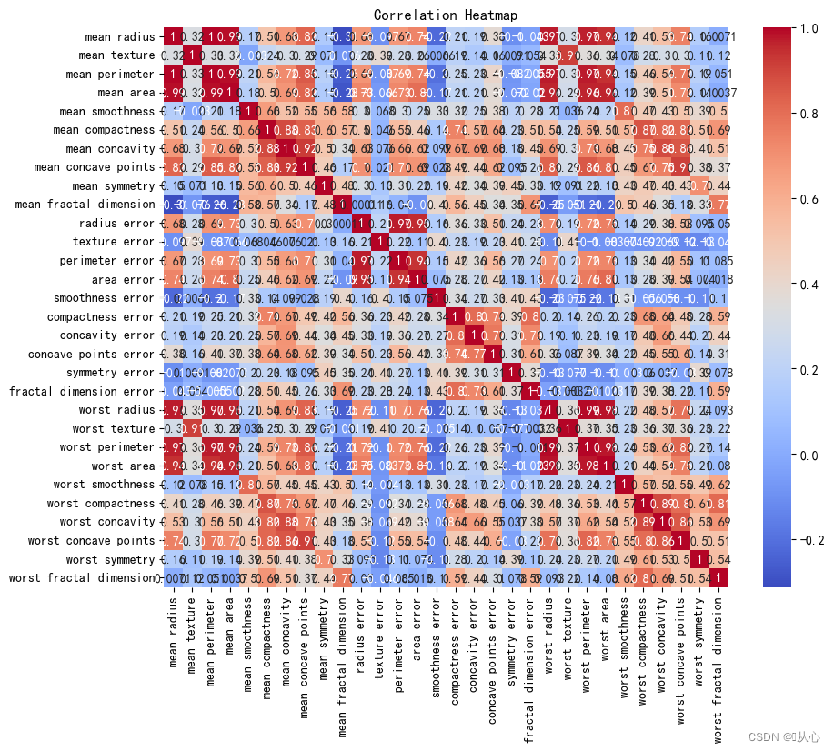
- # 计算相关系数
- correlation_matrix = df.corr()
-
- # 可视化相关系数热力图
- plt.figure(figsize=(10, 8))
- sns.heatmap(correlation_matrix, annot=True, cmap="coolwarm")
- plt.title("Correlation Heatmap")
- plt.show()
 2、API
2、API- sklearn.linear_model.LogisticRegression
-
- 导入:
- from sklearn.linear_model import LogisticRegression
-
- 语法:
- LogisticRegression(solver='liblinear', penalty=‘l2’, C = 1.0)
- solver可选参数:{'liblinear', 'sag', 'saga','newton-cg', 'lbfgs'},
- 默认: 'liblinear';用于优化问题的算法。
- 对于小数据集来说,“liblinear”是个不错的选择,而“sag”和'saga'对于大型数据集会更快。
- 对于多类问题,只有'newton-cg', 'sag', 'saga'和'lbfgs'可以处理多项损失;“liblinear”仅限于“one-versus-rest”分类。
- penalty:正则化的种类
- C:正则化力度
- from sklearn.datasets import load_breast_cancer
- from sklearn.model_selection import train_test_split
-
- from sklearn.linear_model import LogisticRegression
-
- # 获取数据
- breast_cancer = load_breast_cancer()
- # 划分数据集
- x_train,x_test,y_train,y_test = train_test_split(breast_cancer.data, breast_cancer.target, test_size=0.2, random_state=1473)
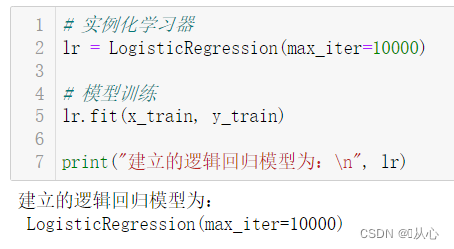
- # 实例化学习器
- lr = LogisticRegression(max_iter=10000)
-
- # 模型训练
- lr.fit(x_train, y_train)
-
- print("建立的逻辑回归模型为:n", lr)
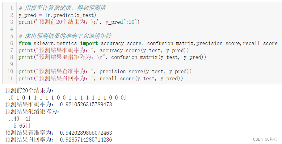
- # 用模型计算测试值,得到预测值
- y_pred = lr.predict(x_test)
- print('预测前20个结果为:n', y_pred[:20])
-
- # 求出预测结果的准确率和混淆矩阵
- from sklearn.metrics import accuracy_score, confusion_matrix,precision_score,recall_score
- print("预测结果准确率为:", accuracy_score(y_test, y_pred))
- print("预测结果混淆矩阵为:n", confusion_matrix(y_test, y_pred))
-
- print("预测结果查准率为:", precision_score(y_test, y_pred))
- print("预测结果召回率为:", recall_score(y_test, y_pred))
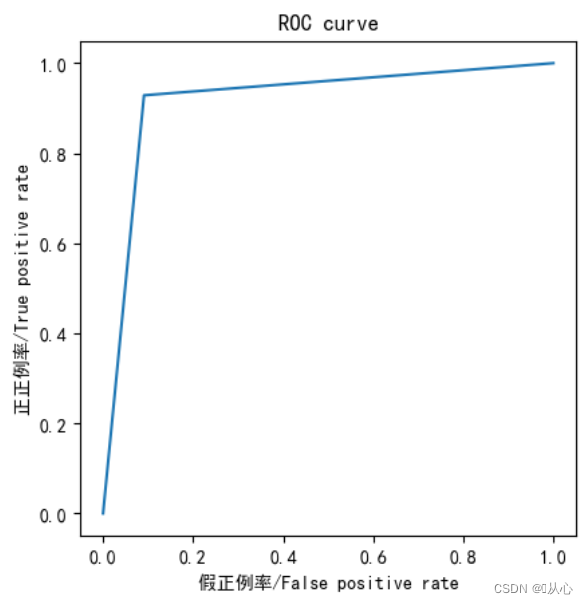
- from sklearn.metrics import roc_curve,roc_auc_score,auc
-
- fpr,tpr,thresholds=roc_curve(y_test,y_pred)
-
- plt.plot(fpr, tpr)
- plt.axis("square")
- plt.xlabel("假正例率/False positive rate")
- plt.ylabel("正正例率/True positive rate")
- plt.title("ROC curve")
- plt.show()
-
- print("AUC指标为:",roc_auc_score(y_test,y_pred))
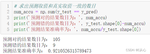
- # 求出预测取值和真实取值一致的数目
- num_accu = np.sum(y_test == y_pred)
- print('预测对的结果数目为:', num_accu)
- print('预测错的结果数目为:', y_test.shape[0]-num_accu)
- print('预测结果准确率为:', num_accu/y_test.shape[0])
After the model evaluation, the model that passes can be substituted into the true value for prediction.
Old dreams can be revisited, and see:Machine Learning (V) -- Supervised Learning (5) -- Linear Regression 2
To know what happened next, please see:Machine Learning (V) -- Supervised Learning (7) -- SVM1

I have devoted myself to the research of technology for more than 30 years. I am proficient in various languages such as Java, Linux, JavaScript, PHP, CSS, etc. I have made many contributions in the field of open source. I have established a developer documentation site to share some problems in technology development for everyone to read.
