2024-07-12
한어Русский языкEnglishFrançaisIndonesianSanskrit日本語DeutschPortuguêsΕλληνικάespañolItalianoSuomalainenLatina
This week, I read a paper titled Interpretable CEEMDAN-FE-LSTM-transformer hybrid model for predicting total phosphorus concentrations in surface water. The paper proposes a hybrid model for TP prediction. The paper proposes a hybrid model for TP prediction, namely the CF-LT model. The model innovatively combines the full integrated empirical mode decomposition (EMD) with adaptive noise processing, fuzzy entropy analysis, long short-term memory network (LSTM) and Transformer technology. By introducing data frequency division and reconstruction technology, the model effectively solves the overfitting and underfitting problems that traditional machine learning models are prone to when processing high-dimensional data. At the same time, the application of the attention mechanism enables the CF-LT model to overcome the limitation of other models that it is difficult to establish long-term dependencies between data when making long-term predictions. The prediction results show that the CF-LT model achieved a determination coefficient (R2) of 0.37 to 0.87 on the test data set, which is a significant improvement of 0.05 to 0.17 (i.e. 6% to 85%) compared with the control model. In addition, the CF-LT model also showed the best peak prediction performance.
This week’s weekly newspaper decodes the paper entitled Interpretable CEEMDAN-FE-LSTM-transformer hybrid model for predicting total phosphorus concentrations in surface water. This paper introduces a hybrid model, CF-LT, specifically for TP prediction. The model innovatively integrates Complete Ensemble Empirical Mode Decomposition (EMD) with adaptive noise processing, fuzzy entropy analysis, Long Short-Term Memory (LSTM) networks, and Transformer technology. By introducing data frequency division and reconstruction, CF-LT effectively addresses the issues of overfitting and underfitting that traditional machine learning models often encounter when dealing with high-dimensional data. Additionally, the application of the attention mechanism enables CF-LT to overcome the limitations of other models in establishing long-term dependencies between data points during long-term predictions. The prediction results demonstrate that CF-LT achieves a decision coefficient (R2) ranging from 0.37 to 0.87 on the test datasets, representing a significant improvement of 0.05 to 0.17 (or 6% to 85%) compared to the control models. Furthermore, CF-LT provides the best peak prediction performance.
标题:Interpretable CEEMDAN-FE-LSTM-transformer hybrid model for predicting total phosphorus concentrations in surface water
Author: Jiefu Yao, Shuai Chen, Xiaohong Ruan
release:Journal of Hydrology Volume 629, February 2024, 130609
链接:https://www.sciencedirect.com/science/article/pii/S0022169424000039?via%3Dihub
This paper proposes a hybrid model for TP prediction. The model (CF-LT) combines the full ensemble empirical mode decomposition (EMD) with adaptive noise, fuzzy entropy, long short-term memory and Transformer.Data frequency division and reconstructionThe introduction of effectively solves the overfitting and underfitting problems that occurred in previous machine learning models when facing high-dimensional data.Attention MechanismThe problem that these models cannot establish long-term dependencies between data is overcome in long-term prediction. The prediction results show that the CF-LT model achieves a coefficient of determination (R2) of 0.37-0.87 on the test data set, which is 0.05-0.17 (6%-85%) higher than the control model. In addition, the CF-LT model provides the best peak prediction.
As an advanced time series analysis method, CEEMDAN effectively reduces the mode aliasing problem existing in traditional empirical mode decomposition (EMD) by adding adaptive noise in the EMD process. It can decompose the original signal into a series of intrinsic mode functions (IMFs), each of which represents the different time scale characteristics of the signal, making the analysis of complex signals more intuitive and accurate. In this study, CEEMDAN was used to process daily water quality data from three monitoring stations in Lake Tai, separating total phosphorus concentration and other water quality parameters such as water temperature, pH value, dissolved oxygen, etc. into signals of different frequency bands.
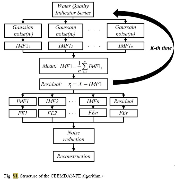
Algorithm S1: Complete Ensemble Empirical Mode Decomposition with Adaptive Noise (CEEMDAN)
y i ( t ) = y ( t ) + ϵ 0 v i ( t ) i = 1 , 2 , … , n (S1) y^{i}(t)=y(t)+epsilon_0v^i(t)quad i=1,2,dots,ntag{S1} yi(t)=y(t)+ϵ0vi(t)i=1,2,…,n(S1)
IMF1 i = E 0 ( y i ( t ) ) + r 1 i IMF1 ‾ = 1 n IMF1 i (S2) text{IMF1}_i=E_0(y^i(t))+r^i_1quad overline{text{IMF1}}=frac1ntext{IMF1}_itag{S2} IMF1i=E0(yi(t))+r1iIMF1=n1IMF1i(S2)
r 1 = y i ( t ) − IMF1 ‾ (S3) r_1=y^i(t)-overline{text{IMF1}}tag{S3} r1=yi(t)−IMF1(S3)
IMF2 ‾ = 1 n ∑ i = 1 n E 1 ( r 1 + ϵ 1 E 1 ( v i ( t ) ) ) (S4) overline{text{IMF2}}=frac1nsum^n_{i=1}E_1(r_1+epsilon_1E_1(v^i(t))) tag{S4} IMF2=n1i=1∑nE1(r1+ϵ1E1(vi(t)))(S4)
y ( t ) = ∑ l = 1 K − 1 IMF1 ‾ + r K (S5) y(t)=sum^{K-1}_{l=1}overline{text{IMF1}}+r_Ktag{S5} y(t)=l=1∑K−1IMF1+rK(S5)
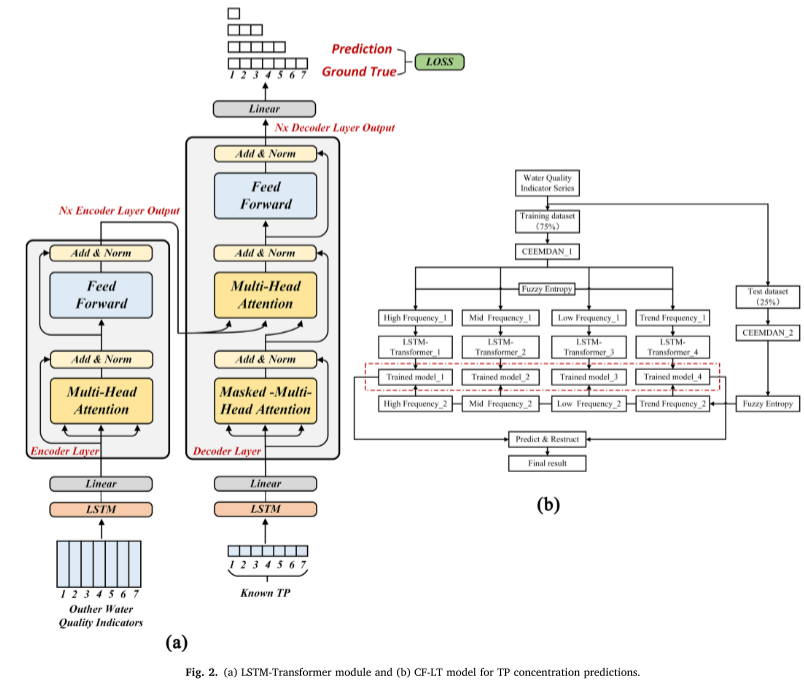
For the CEEMDAN-FE part, we first divide the original dataset into training and testing datasets, and then apply CEEMDAN to decompose each feature in the two datasets into multiple intrinsic mode functions (IMFs). According to the proximity of the FE values of each IMF, they are reconstructed into high-frequency (IMFH), medium-frequency (IMFM), low-frequency (IMFL), and trend term (IMFT) components, which reflect different aspects of IMF.
For the LSTM-Transformer part, in the encoder and decoder, the hidden layer of LSTM is replaced by Transformer position encoding to establish the temporal dependency between input data. The specific calculation process is as follows (Figure 2a).
SHAP is a game theory method for explaining the output of any ML model. To determine the impact of input features on the model output, the input features
z
=
[
z
1
,
.
.
.
,
z
p
]
z = [z1, ..., zp]
z=[z1,...,zp] is associated with the trained deep learning model F.
F
=
f
(
z
)
=
ϕ
0
+
∑
i
=
1
M
ϕ
i
z
i
(12)
F=f(z)=phi_0+sum_{i=1}^M phi_iz_i tag{12}
F=f(z)=ϕ0+i=1∑Mϕizi(12)
φ
i
∈
R
φ_i ∈ R
φi∈RIt represents the contribution of each feature to the model, which is given by the following formula:
ϕ
i
(
F
,
x
)
=
∑
z
≤
x
∣
z
∣
!
(
M
−
∣
z
∣
−
1
)
!
M
!
[
F
(
z
)
−
F
(
z
/
i
)
]
(13)
phi_i(F,x)=sum_{zleq x}frac{|z|!(M-|z|-1)!}{M!}[F(z)-F(z/i)] tag{13}
ϕi(F,x)=z≤x∑M!∣z∣!(M−∣z∣−1)
This study proposes a new model for predicting total phosphorus concentration. The model combines CEEM DAN, FE, LSTM and Transformer techniques, and uses SHAP to interpret the model output. The main objectives of this study are to evaluate the performance of the proposed CEEMDAN-FE-LSTM-Transformer (CF-LT) model in predicting TP concentrations at the entrance of Taihu Lake and apply SHAP to interpret the output of the CF-LT model. This should reveal the key factors affecting TP concentrations in the region and their response mechanisms.
Decomposition of high-dimensional data may produce a large number of modal components. To address this problem, Fuzzy Entropy (FE), an efficient method with low computational time complexity, can be combined with CEEMDAN. This combination effectively reconstructs the sub-signals after CEEMDAN decomposition, thereby reducing the number of sub-frequency models.
The LSTM Transformer model can capture the relationship between non-adjacent time points while preserving the time series characteristics of the input data.
The Transformer model uses an attention mechanism to identify the correlation between two positions in a specific context during training. This enables efficient acquisition of relevant data and reduces information redundancy.
The main contributions of this paper are fourfold:
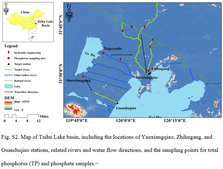
data set:The Taihu Lake Basin is located in the lower reaches of the Yangtze River, covering an area of 36,900 square kilometers, with a dense river network and numerous lakes. Taihu Lake is a typical shallow lake. The basin has the characteristics of a northern subtropical humid climate, with an average annual temperature of 15-17°C and an average annual precipitation of 1181 mm. This study used water quality monitoring data from Yaoxiangqiao Station, Zhihugang Station, and Guanduqiao Station (Figure S2). These monitoring stations are located at the Taihukou, a national key water quality assessment section. The data comes from the Jiangsu Provincial Environmental Monitoring Center.
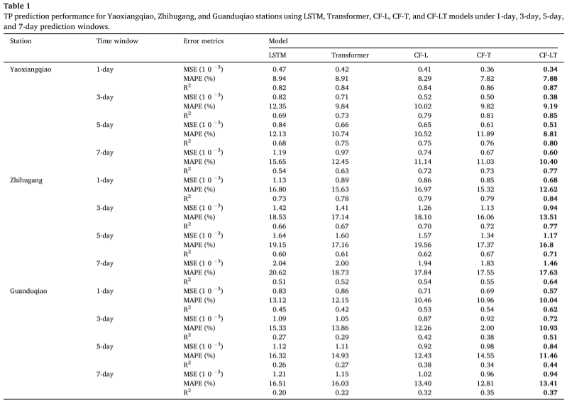
Evaluation Criteria:The performance evaluation of the model uses several key indicators: determination coefficient (R²), mean square error (MSE), and mean absolute percentage error (MAPE). R² measures the degree of fit between the model prediction value and the actual value. A value close to 1 indicates that the model has strong prediction ability; MSE measures the sum of squares of prediction errors. The smaller the value, the smaller the prediction error; MAPE reflects the size of the prediction error from a percentage perspective. The lower the value, the more accurate the prediction.
Implementation details:The experimental process includes data preprocessing, model training and testing. A complete experimental procedure is established to evaluate the performance of the proposed model on different datasets and prediction time windows. First, the data is preprocessed by the CEEMDAN-FE method, and the fully integrated empirical mode decomposition with adaptive noise is added to remove information interference, extract multi-scale information, and reduce the number of sub-signals using fuzzy entropy. Then, the processed data is divided into training and test sets with a ratio of 75% and 25%. In the training phase, the preprocessed training dataset is input to the LSTM-Transformer model. Back-propagation and Adam optimizer are used to update the model weights, and grid search is adopted to identify the optimal hyperparameters of the LSTMTransformer module to ensure the best performance of the model under different prediction time windows (7 days, 5 days, 3 days, 1 day).
Experimental Results : The best trained model was applied to the test dataset, and the table summarizes the TP concentration predictions given by the CF-LT, LSTM, Transformer, CF-L, and CF-T models at different sites and different prediction time windows. The proposed CF-LT model gave the best results for all three evaluation metrics. In terms of R2, the CF-LT model ranged from 0.37 to 0.87, while the next best CF-L and CF-T models were 0.32-0.84 and 0.35-0.86, respectively. This suggests that combining the long-term memory of LSTM with the attention mechanism of Transformer can improve the prediction accuracy. Comparing the worst LSTM and Transformer models with the CF-L and CF-T models, the MAPE ranges from 8.94%-20.62% (LSTM) and 8.91%-18.73% (Transformer) to 8.29%-19.56% (CF-L) and 7.82%-17.55% (CF-T). These results indicate that data decomposition and frequency-decomposition modeling significantly improve prediction accuracy by capturing more information hidden in the original data.
Prediction of factors affecting total phosphorus TP concentration:
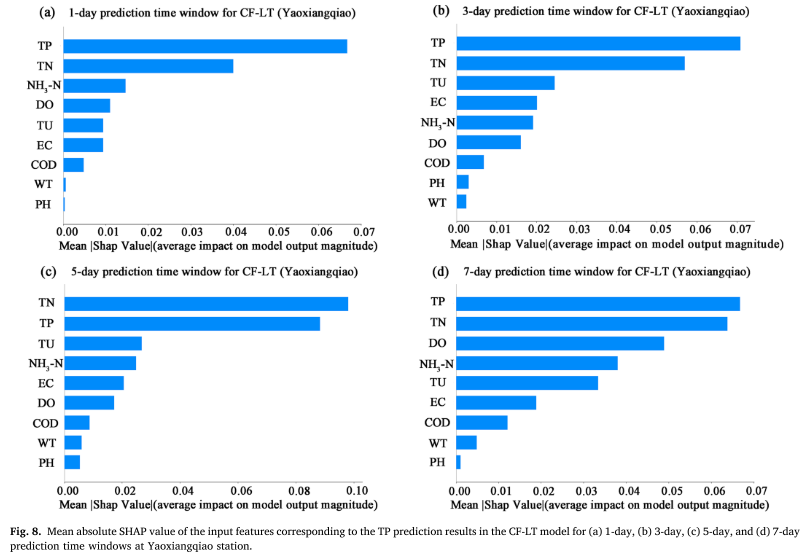
The mean absolute SHAP value (MASV) was used to quantify the contribution of input features (WT, PH, DO, COD, EC, TU, TN, NH3-N, TP) to TP prediction results. The larger the MASV, the greater the impact on the model prediction results. The study showed that in addition to the past TP concentration series itself, total nitrogen (TN) and turbidity (TU) are the two main factors affecting TP prediction. This shows that the change of TP is not only directly affected by historical concentrations, but also closely related to non-point source pollution emissions and algal growth dynamics associated with nitrogen-phosphorus ratios in water bodies. In particular, the significant correlation between TN and TP emphasizes the coupling effect of the two in the nutrient cycle of lakes, highlighting the importance of non-point source nitrogen inputs for phosphorus concentration prediction.
From these results, the following observations can be made:
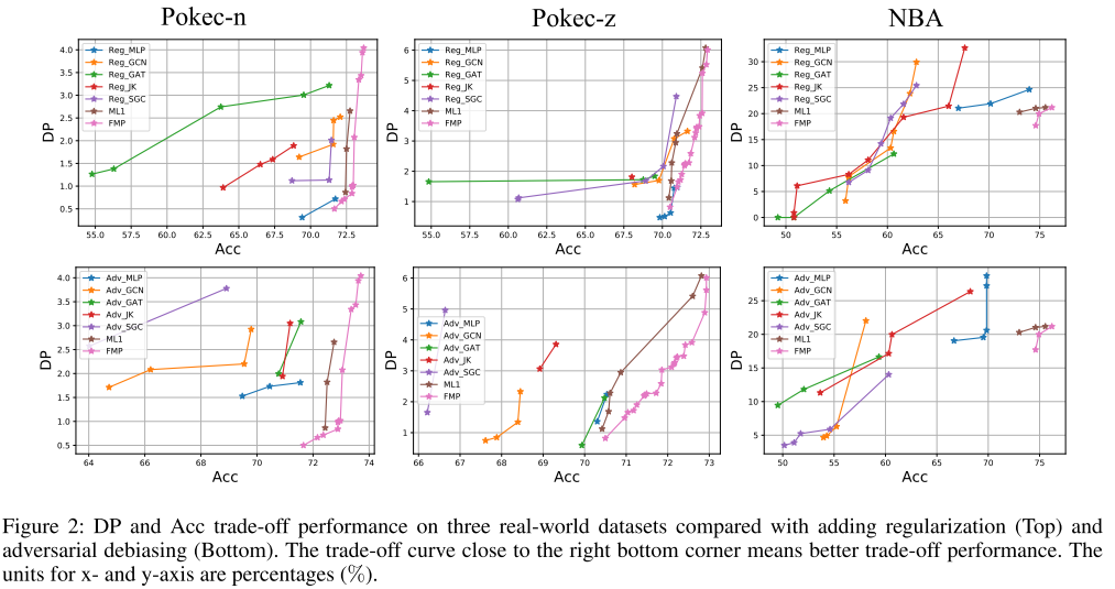
Comparison with Adversarial Debiasing and Regularization: Randomly split 50%/25%/25% for training, validation, and testing datasets. Figure 2 shows the Pareto optimality curves for all methods, where the lower right corner point represents the ideal performance (highest accuracy and lowest prediction bias).
The CF-LT hybrid model proposed in this paper combines CEEM DAN, FE, LSTM and Transformer modules to predict TP concentrations in surface water. This hybrid approach solves the shortcomings of model overfitting and underfitting caused by high-dimensional data and the inability to establish long-term dependencies between data when making long-term predictions. In addition, SHAP values are used to explain the output of the CF-LT model.
The model applies data from three water quality monitoring stations in the Taihu Lake Basin and outputs nine water quality indicators for different prediction time windows. LSTM, Transformer, CF-L, and CF-T algorithms were used as control models. The CF-LT model had an R2 value of 0.37–0.87, an MSE value of 0.34 × 10⁻³–1.46 × 10⁻³, and a MAPE value of 7.88%-17.63% on the test dataset, indicating that all three indicators were better than the LSTM, Transformer, CF-L, and CF-T results. The proposed CF-LT model also produced the best peak prediction results. Based on the SHAP explanation, we found that TU and TN (excluding the early time series of TP concentration) were important factors affecting TP prediction, indicating that the change of TP was not only related to the early level of TP concentration, but also affected by TP concentration. Relationship between non-point source pollution emissions and N and P of aquatic plants at the Taihu estuary. In addition, it is worth noting that TN and TU contributed more to the prediction of TP concentration in the rainy season. Therefore, the results of this study suggest that the CF-LT model provides additional information for understanding the response mechanism of TP under changing environmental conditions.
CEEMDAN and FE data preprocessing
def ceemdan_fe_preprocessing(data):
    # CEEMDAN分解
    imfs, residue = ceemdan(data, **ceemdan_params)

    # 计算各个IMF的模糊熵
    fe_values = []
    for imf in imfs:
        fe_values.append(fuzzy_entropy(imf)) # 假定fuzzy_entropy为计算模糊熵的函数

    # 根据FE值重组IMFs
    imfs_sorted = [imf for _, imf in sorted(zip(fe_values, imfs))]
    imf_hf, imf_mf, imf_lf, imf_trend = imfs_sorted[:4], imfs_sorted[4:8], imfs_sorted[8:12], imfs_sorted[12:]
    return np.concatenate((imf_hf, imf_mf, imf_lf, imf_trend), axis=1)

# 应用到数据上
preprocessed_data = ceemdan_fe_preprocessing(original_data)
LSTM&Transformer
def get_positional_encoding(max_len, d_model):
    pe = np.zeros((max_len, d_model))
    position = np.arange(0, max_len).reshape(-1, 1)
    div_term = np.exp(np.arange(0, d_model, 2) * -(np.log(10000.0) / d_model))
    pe[:, 0::2] = np.sin(position * div_term)
    pe[:, 1::2] = np.cos(position * div_term)
    return pe

def transformer_encoder(inputs, d_model, num_heads, ff_dim):
    x = MultiHeadAttention(num_heads=num_heads, key_dim=d_model)(inputs, inputs)
    x = LayerNormalization()(Add()([inputs, x]))
    x = Dense(ff_dim, activation='relu')(x)
    x = Dense(d_model)(x)
    x = LayerNormalization()(Add()([inputs, x]))
    return x

def transformer_decoder(inputs, encoder_outputs, d_model, num_heads, ff_dim):
    return decoder_output

input_features = Input(shape=(input_shape))
lstm_out = LSTM(lstm_units)(input_features) # LSTM

pos_encodings = get_positional_encoding(max_seq_length, d_model)

transformer_in = Add()([lstm_out, pos_encodings])
transformer_encoded = transformer_encoder(transformer_in, d_model, num_heads, ff_dim)

decoder_output = transformer_decoder(decoder_input, transformer_encoded, d_model, num_heads, ff_dim)

output_layer = Dense(output_dim, activation='linear')(decoder_output)
model = Model(inputs=input_features, outputs=output_layer)

model.compile(optimizer=Adam(learning_rate), loss='mse')
This study developed an interpretable CEEMDAN-FE-LSTM-Transformer hybrid model for the prediction of total phosphorus concentration in surface water. The model significantly improved the prediction accuracy through the integration of advanced data preprocessing technology and deep learning models, and provided clear feature interpretation through SHAP. The experimental results confirmed the effectiveness of the model, especially the identification of key environmental factors, which provides a powerful tool for eutrophication management and pollution control of water bodies.
[1] Jiefu Yao, Shuai Chen, Xiaohong Ruan. Interpretable CEEMDAN-FE-LSTM-transformer hybrid model for predicting total phosphorus concentrations in surface water. [J] Journal of Hydrology Volume 629, February 2024, 130609

I have devoted myself to the research of technology for more than 30 years. I am proficient in various languages such as Java, Linux, JavaScript, PHP, CSS, etc. I have made many contributions in the field of open source. I have established a developer documentation site to share some problems in technology development for everyone to read.

