2024-07-12
한어Русский языкEnglishFrançaisIndonesianSanskrit日本語DeutschPortuguêsΕλληνικάespañolItalianoSuomalainenLatina
The vector database is the core component of today's large-model knowledge base retrieval implementation. The following figure is the architecture diagram for building knowledge base retrieval: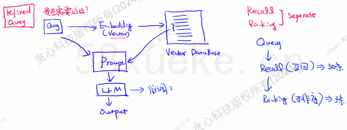
The similarity between the vector query data and the query directly affects the quality of the prompt. This article will briefly introduce the existing vector databases on the market, and then explain the indexing methods used, including inverted index, KNN, Approximate KNN, Product Quantization, HSNW, etc., and explain the design concepts and methods of these algorithms.
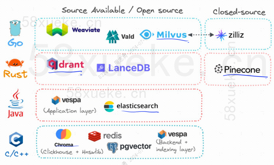
The three most popular open source vector databases are Chroma, Milvus, and Weaviate. I think this article is good about their introduction and differences. If you are interested, you can take a look:Comparison of the three major open source vector databases。
The following is the development history of open source vector databases: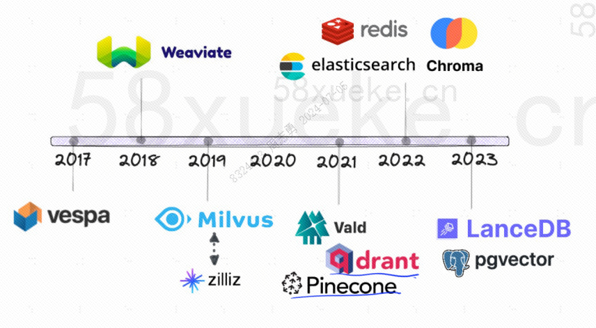
The indexing methods they use are as follows: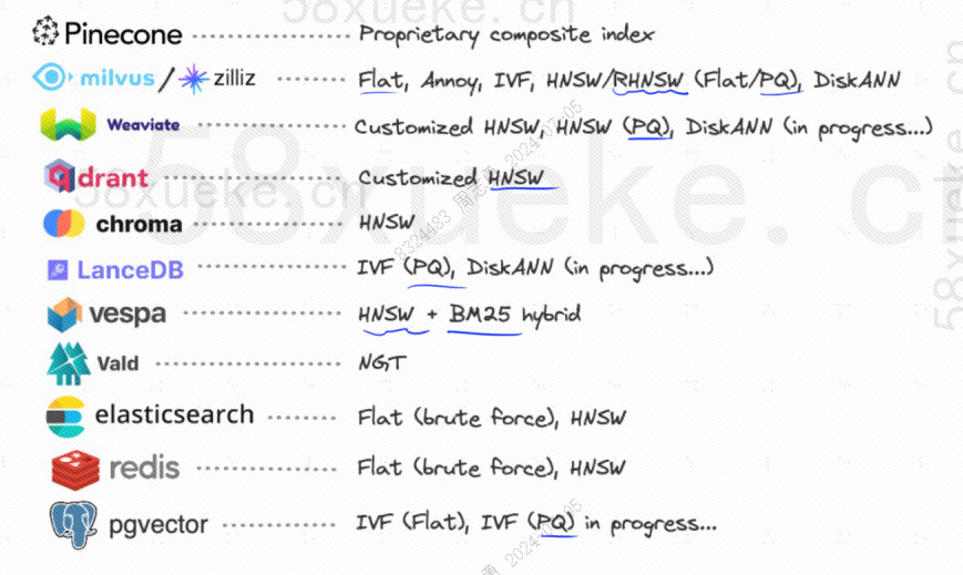
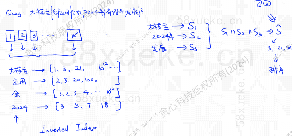
Suppose I have a database using an inverted index, which stores 10 to the 12th power of index data. When we store data in the database, we will segment the data and then record the index positions corresponding to the segmented words. Because the same words may appear in different sentences, each word corresponds to an index set:
Suppose now I have a query: What developments will the application of large models have in 2024?
The database divides our query into three keywords: big model, 2024, and development. Then it finds the index combination corresponding to each word and finds the intersection. This query process is calledrecall.
At this point, we have obtained the data associated with the query, but the similarity between these data and the query statement is different. We need to sort them and take the TOP N.
However, this query that directly matches text data with indexes is not very efficient. Is there any way we can speed up similarity retrieval?
At this time, vectorized retrieval appears, which converts data into vectors and then calculates the vectorSimilarityanddistanceThere are two ways to search: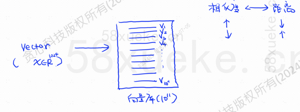
KNN search is called K nearest neighbor search. It converts the query statement into a vector and then compares the vector with the vector in the database.Highest similarity, closest distanceVector set.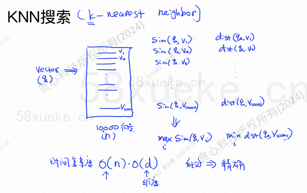
The time complexity is O(N)*O(d), where d is the dimension. The dimension data is generally fixed. Assuming that there are 10,000 vector data stored in the database, and the dimension is 1024, then the query maxSim(q,v)(highest similarity),minDist(q,v)The time complexity of the (closest) vector is O(10000)*O(1024).
The advantage of this retrieval method is that the data retrieved is highly accurate, but the disadvantage is that it is slow.
Approximate KNN search is to change the search space from points to blocks, first determine the closest block, and then find the closest point with the highest similarity in the block space. The left side of the figure below is KNN search, and the side is approximate KNN search: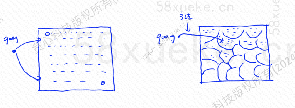
Each block has a center point. Calculating the distance between the query point and the block is to calculate the distance from the query point to the center point of each block: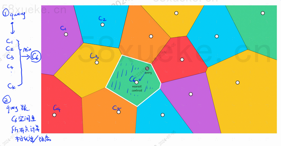
For example, the query steps in the figure above are as follows:
However, we can see with our naked eyes that although the center points of the red and orange blocks are far from the query point, the points in their blocks are close to the query point. At this time, we need to expand the range of the search block: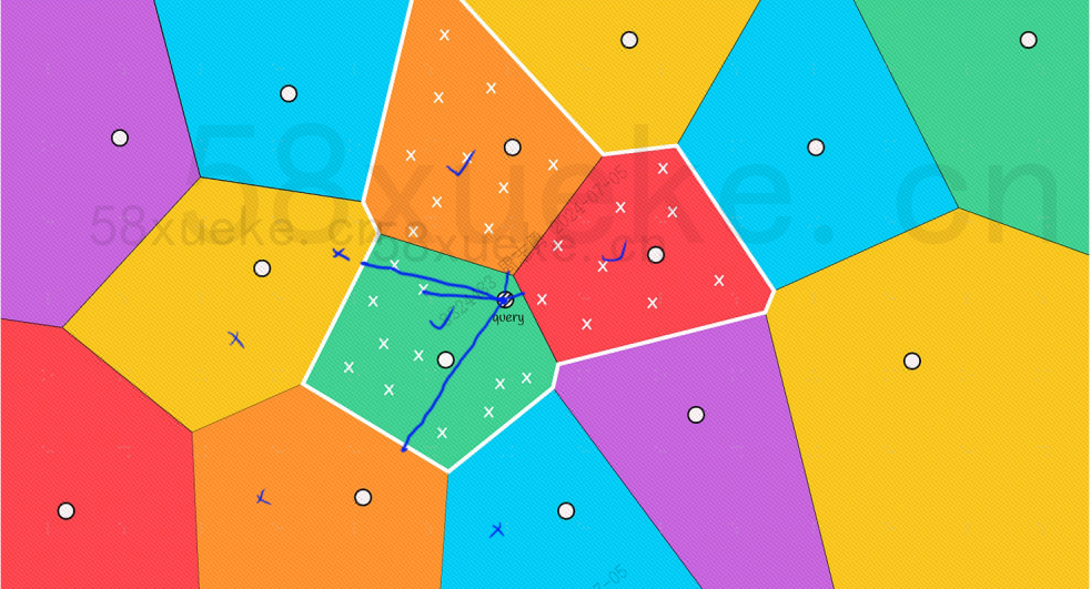
Below is the algorithm formula for finding the highest similarity and the closest distance. The highest similarity (COS_SIM) is calculated by cosine, and there are two algorithms for the closest distance, the Euclidean algorithm and the Manhattan algorithm, which will not be explained here: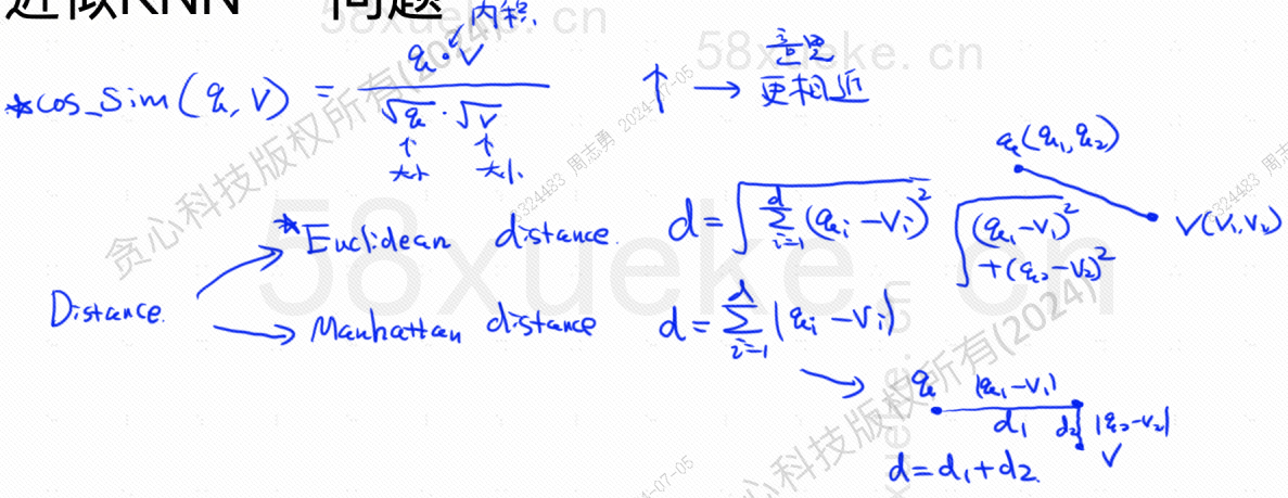
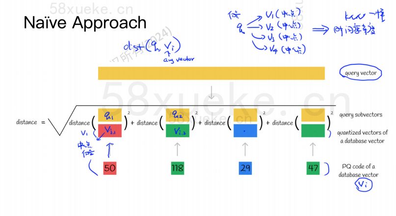
The PQ algorithm first divides all vectors into multiple subspaces. Like the approximate KNN, each subspace has a centroid.
The original high-dimensional vector is then split into multiple low-dimensional sub-vectors, and the center point closest to the sub-vector is used as the PQ ID of the sub-vector. Then a high-dimensional vector is composed of multiple PQ IDs, which greatly compresses the space.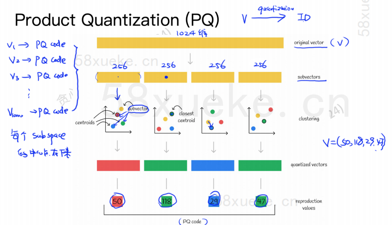
For example, the 1024-dimensional vector in the figure above is split into four 256-dimensional sub-vectors, and the four sub-vectors are closest to the center points: 50, 118, 29, and 47. Therefore, the 1024-dimensional vector can be represented by V=(50, 118, 29, 47), and its PQ code is also (50, 118, 29, 47).
Therefore, the vector database using the PQ algorithm needs to save the information of all center points and the PQ codes of all high-dimensional vectors.
Suppose we have a query statement that requires us to find the vector with the highest similarity from the vector database. How do we use the PQ algorithm to find the vector?
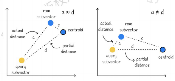
The one on the left is a case with very small errors, and the one on the right is a case with relatively large errors. Generally there will be a few errors, but most of the errors are relatively small.
Using caching to speed up calculations
If the original query vector and the PQ code of each subvector need to be calculated once, then it is not much different from the approximate KNN algorithm, and the space complexity is O(n)*O(k). So what is the meaning of this algorithm? Is it just for compression and reducing space storage?
Assume that all vectors are divided into K subspaces, each of which has n points. We calculate the distance from each point in each subspace to its center point in advance and put it into a two-dimensional matrix. Then we can query the distance from each subvector corresponding to the vector to the center point directly from the matrix, as shown in the following figure: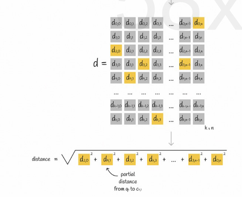
Finally, we just need to add the distance of each subvector and take the square root.
Combining approximate KNN with PQ algorithm
These two algorithms are not conflicting. You can first use approximate KNN to divide all vectors into multiple subspaces, and then locate the query vector in the corresponding subspace.
In this way, the PQ algorithm is used in the subspace to speed up the calculation.
In a given vector data set, according to a certain metric, K vectors close to the query vector are retrieved (K-Nearest Neighbor, KNN). However, due to the large amount of calculation of KNN, we usually only focus on the approximate nearest neighbor (ANN) problem.
When NSW constructs a graph, it randomly selects points and adds them to the graph. Each time a point is added, it searches for its nearest m points to add edges. Finally, the structure shown in the following figure is formed:
When searching the NSW graph, we start from a predefined entry point. This entry point is connected to several nearby vertices. We determine which of these vertices is closest to our query vector and move there.
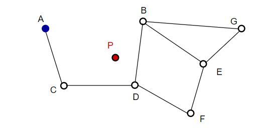
For example, starting from A, A's neighbor point C is closer to P and is updated. Then C's neighbor point D is closer to P, and then D's neighbor points B and F are not closer, so the program stops and the point is D.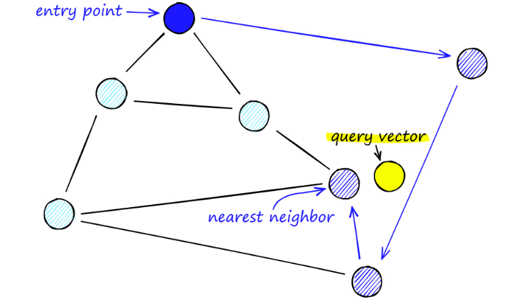
The construction of the graph starts from the top level. After entering the graph, the algorithm greedily traverses the edges and finds the closest ef neighbor to the vector q we inserted - at this time ef = 1.
After finding the local minimum, it moves down to the next layer (just as it did during the search). This process repeats until it reaches the insertion layer of our choice. Here begins the second phase of construction.
The ef value increases to the efConstruction parameter we set, which means that more nearest neighbors will be returned. In the second phase, these nearest neighbors are candidates for links to the newly inserted element q and serve as entry points to the next layer.
After multiple iterations, two more parameters are considered when adding links: M_max, which defines the maximum number of links a vertex can have, and similarly M_max0, which defines the maximum number of connections for vertices in level 0.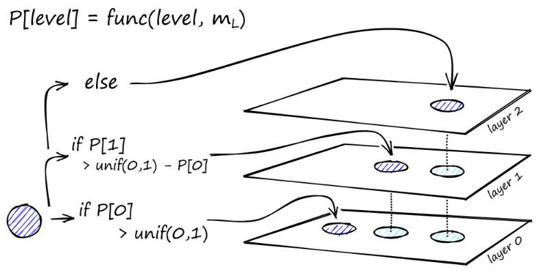
HNSW stands for Hierarchical Navigable Small World, a multi-layered graph. Every object in the database is captured in the lowest layer (layer 0 in the picture). These data objects are well connected. On each layer above the lowest layer, fewer data points are represented. These data points match the lower layers, but there are exponentially fewer points in each higher layer. If there is a search query, the closest data point will be found in the highest layer. In the example below, this is just one more data point. Then it goes one layer deeper and finds the closest data point from the first found data point in the highest layer and searches for the nearest neighbors from there. At the deepest layer, the actual data object closest to the search query will be found.
HNSW is a very fast and memory-efficient similarity search method because only the highest layer (top layer) is kept in cache instead of all data points in the lowest layer. Only the data points closest to the search query are loaded after being requested by a higher layer, which means that only a small amount of memory needs to be kept.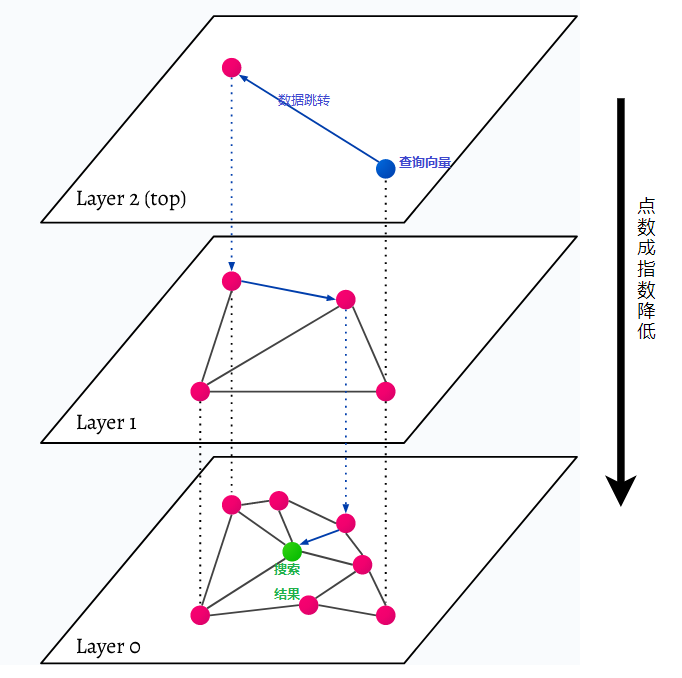

I have devoted myself to the research of technology for more than 30 years. I am proficient in various languages such as Java, Linux, JavaScript, PHP, CSS, etc. I have made many contributions in the field of open source. I have established a developer documentation site to share some problems in technology development for everyone to read.
