2024-07-12
한어Русский языкEnglishFrançaisIndonesianSanskrit日本語DeutschPortuguêsΕλληνικάespañolItalianoSuomalainenLatina
The COVID-19 epidemic has touched the hearts of each of us. In this case, we will try to use social computing methods to analyze news and rumors related to the epidemic and helpEpidemic InformationResearch. This assignment is an open assignment. We provide social data during the epidemic and encourage students to analyze social trends from news, rumors, and legal documents. (Hint: Use the methods learned in class, such as sentiment analysis, information extraction, reading comprehension, etc. to analyze data)
https://covid19.thunlp.org/ provides social data information related to the COVID-19 pandemic, including rumors related to the pandemic (CSDC-Rumor), Chinese news related to the pandemic (CSDC-News), and legal documents related to the pandemic (CSDC-Legal).
This part of the dataset collects:
(1) Starting from January 22, 2020False information on WeiboData, including the content, publisher, reporter, trial time, and results of microblogs identified as false information. As of March 1, 2020, there were 324 original microblogs, 31,284 reposts, and 7,912 comments, which will be used to help researchers analyze and study the spread of false information during the epidemic.
(2) Tencent rumor verification platform and DXY false information data starting from January 18, 2020, including the content of rumors that were determined to be correct or false, the time, and the basis for judging whether it was a rumor. As of March 1, 2020, there were 507 rumor data in total, including 124 factual data, with the data distribution as follows: negative examples: 420, positive examples: 33, and uncertain examples: 54.
This part of the dataset collects news data starting from January 1, 2020, including news titles, content, keywords, and other information. As of March 16, 2020, a total of 148,960 news items and 1,653,086 corresponding comments were collected to help researchers analyze and study news data during the epidemic.
This data is for CAIL A total of 1,203 pieces of historically relevant legal documents were selected from the anonymized legal document data collected. Each piece of data contains the document title, case number, and full text of the document for researchers to use in their research on legal issues related to the epidemic.
This assignment is an open assignment.
Grade the assignments in terms of aspects.
[1] Information credibility on twitter. in Proceedings of WWW, 2011.
[2] Detecting rumors from microblogs with recurrent neural networks. in Proceedings of IJCAI, 2016.
[3] A convolutional approach for misinformation identification. in Proceedings of IJCAI, 2017.
[4] The spread of true and false news online. Science, 2018.
[5] False information on web and social media: A survey. arXiv preprint, 2018.
[6] Characterization of the Affective Norms for English Words by Discrete Emotional Categories. Behavior Research Methods, 2007.
This experiment provides a dataset of epidemic-related rumors, CSDC-Rumor. By analyzing the content of the dataset, we first conduct quantitative statistical analysis on the dataset, then use clustering to implement semantic analysis of rumors, and finally design a rumor detection system.
Data Format
This experiment provides a dataset of epidemic-related rumors, CSDC-Rumor, which collects false information data and rumor-refuting data on Weibo. The dataset contains the following contents.
rumor
│  fact.json
│
├─rumor_forward_comment
│      2020-01-22_K1CaS7Qxd76ol.json
│      2020-01-23_K1CaS7Q1c768i.json
...
│      2020-03-03_K1CaS8wxh6agf.json
└─rumor_weibo
        2020-01-22_K1CaS7Qth660h.json
        2020-01-22_K1CaS7Qxd76ol.json
        ...
        2020-03-03_K1CaS8wxh6agf.json
False information on WeiboRespectively by rumor_weibo andrumor_forward_comment Two names injson The file describes.rumor_weibo middlejson The specific fields are as follows:
rumorCode: The unique code of the rumor, which can be used to directly access the rumor reporting page.title: The title content of the rumor being reported.informerName: The Weibo name of the reporter.informerUrl: Link to the reporter’s Weibo account.rumormongerName: The Weibo name of the person who spread the rumor.rumormongerUr: Link to the Weibo account of the person who spread the rumor.rumorText: Rumor content.visitTimes: Number of times the rumor has been visited.result: The result of review of the rumor.publishTime: The time when the rumor was reported.related_url: Links to evidence, regulations, etc. related to the rumor.rumor_forward_comment middlejson The specific fields are as follows:
uid: Posting user ID.text: Comment or forward with a message.date: release time.comment_or_forward: Binary, either comment, or forward, indicating whether the message is a comment or a forwarded message.Tencent and DXY’s False InformationThe content format is:
date: timeexplain: Rumor Typetag: Rumor Tagsabstract: To verify the content of rumorsrumor: RumorData preprocessing
pass json.load() Extract rumor Weibo data separatelyweibo_data Forwarding data with rumor commentsforward_comment_data , and then convert it to DataFrame format. For files with the same name, Weibo articles correspond to Weibo comments forwarded. When processing the data in the rumor_forward_comment folder, add rumorCode for subsequent matching.
# 文件路径
weibo_dir = 'data/rumor/rumor_weibo'
forward_comment_dir = 'data/rumor/rumor_forward_comment'

# 初始化数据列表
weibo_data = []
forward_comment_data = []

# 处理rumor_weibo文件夹中的数据
for filename in os.listdir(weibo_dir):
    if filename.endswith('.json'):
        filepath = os.path.join(weibo_dir, filename)
        with open(filepath, 'r', encoding='utf-8') as file:
            data = json.load(file)
            weibo_data.append(data)

# 处理rumor_forward_comment文件夹中的数据
for filename in os.listdir(forward_comment_dir):
    if filename.endswith('.json'):
        filepath = os.path.join(forward_comment_dir, filename)
        with open(filepath, 'r', encoding='utf-8') as file:
            data = json.load(file)
            # 提取rumorCode
            rumor_code = filename.split('_')[1].split('.')[0]
            for comment in data:
                comment['rumorCode'] = rumor_code  # 添加rumorCode以便后续匹配
                forward_comment_data.append(comment)

# 转换为DataFrame
weibo_df = pd.DataFrame(weibo_data)
forward_comment_df = pd.DataFrame(forward_comment_data)
This section uses quantitative statistical analysis to provide a specific understanding of the distribution of epidemic rumor Weibo data.
Statistics on the number of visits to rumors
statistics weibo_df['visitTimes'] The number of visits is distributed and the corresponding bar chart is drawn. The results are as follows.
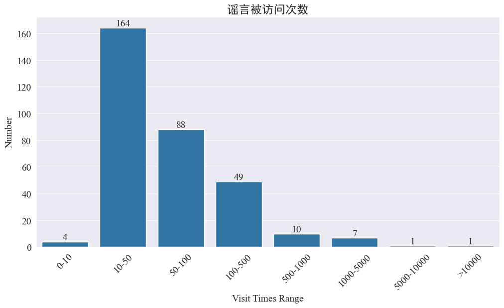
According to the number of visits to Weibo, most of the epidemic rumor Weibo visits are within 500 times, of which 10-50 times account for the largest proportion. However, there are also rumor Weibo visits that are more than 5,000 times, which are considered to have caused serious impacts and have reached the level of "serious circumstances" in law.
Statistics on the number of rumormongers and whistleblowers
By statistics weibo_df['rumormongerName'] andweibo_df['informerName'] The number of rumors spread by each rumor spreader and the number of rumors reported by each reporter are obtained, and the results are as follows.
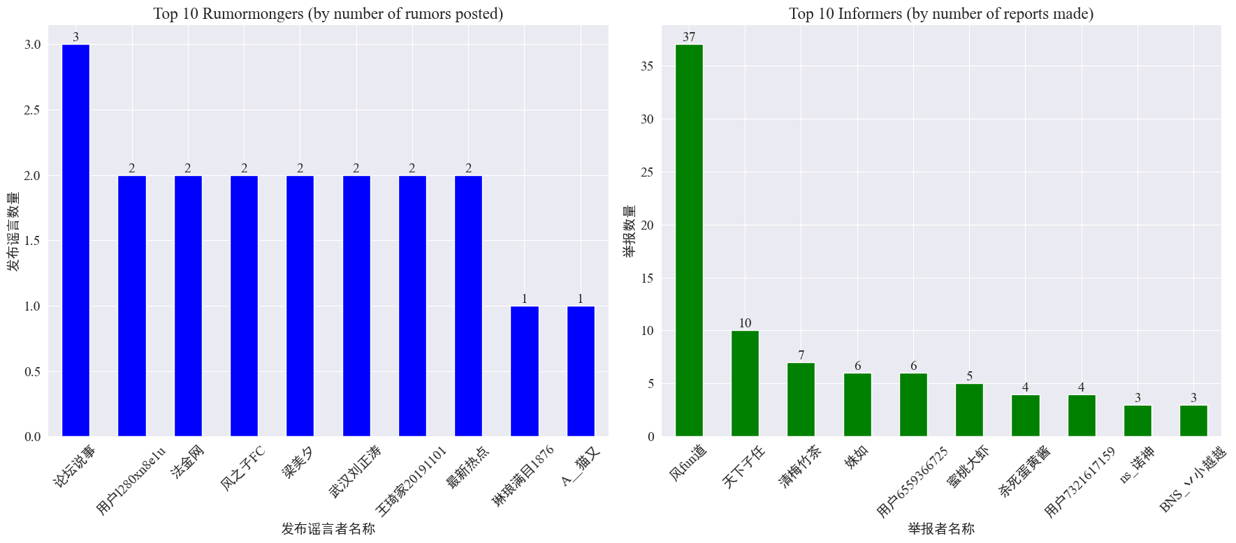
It can be seen that the number of rumors posted by rumor mongers is not concentrated on a few people, but is relatively evenly distributed. The account that posted the most rumors posted 3 rumor Weibo posts. The top 10 reporters each reported at least 3 rumor articles, and the number of rumor Weibo posts reported by reporter Fengfundao was significantly higher than that of other users, reaching 37.
Based on the above data, the audience can focus on reporting accounts that spread a large number of rumors, which facilitates the detection of rumors.
Statistics on the distribution of rumor forwarding and comment volume
By counting the number of rumor forwarding and commenting, we get the following distribution image.

It can be seen that most rumor microblogs have less than 10 comments and reposts, with the maximum number of comments not exceeding 500 and the maximum number of reposts reaching more than 10,000. According to the Internet Management Law, if the number of reposts of a rumor exceeds 500, it is considered a "serious situation".
Cluster analysis of rumor text
This section preprocesses the data of Weibo rumor texts, performs word segmentation, and then conducts cluster analysis to see where Weibo rumors are concentrated.
Data preprocessing
First, the rumor data text is cleaned and the default values are removed. <> The enclosed link content.
# 去除缺失值
weibo_df_rumorText = weibo_df.dropna(subset=['rumorText'])

def clean_text(text):
    # 定义正则表达式模式,匹配 <>
    pattern = re.compile(r'<.*?>')
    # 使用 sub 方法删除匹配的部分
    cleaned_text = re.sub(pattern, '', text)
    return cleaned_text

weibo_df_rumorText['rumorText'] = weibo_df_rumorText['rumorText'].apply(clean_text)
Then load the Chinese stop words, stop words are used cn_stopwords ,usejieba Implement word segmentation of data and perform text vectorization.
# 加载停用词文件
with open('cn_stopwords.txt', encoding='utf-8') as f:
    stopwords = set(f.read().strip().split('n'))

# 分词和去停用词函数
def preprocess_text(text):
    words = jieba.lcut(text)
    words = [word for word in words if word not in stopwords and len(word) > 1]
    return ' '.join(words)

# 应用到数据集
weibo_df_rumorText['processed_text'] = weibo_df_rumorText['rumorText'].apply(preprocess_text)

# 文本向量化
vectorizer = TfidfVectorizer(max_features=10000)
X_tfidf = vectorizer.fit_transform(weibo_df_rumorText['processed_text'])
Determine the best cluster
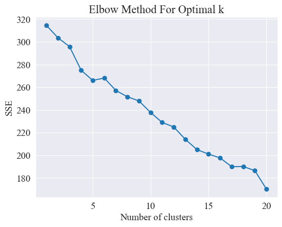
By using the elbow method, the best clustering is determined.
The Elbow Method is a method for determining the optimal number of clusters in cluster analysis. It is based on the relationship between the sum of squared errors (SSE) and the number of clusters. SSE is the sum of the squares of the Euclidean distances from all data points in a cluster to the center of the cluster to which it belongs. It reflects the effect of clustering: the smaller the SSE, the better the clustering effect.
# 使用肘部法确定最佳聚类数量
def plot_elbow_method(X):
    sse = []
    for k in range(1, 21):
        kmeans = KMeans(n_clusters=k, random_state=42, n_init='auto')
        kmeans.fit(X)
        sse.append(kmeans.inertia_)
    plt.plot(range(1, 21), sse, marker='o')
    plt.xlabel('Number of clusters')
    plt.ylabel('SSE')
    plt.title('Elbow Method For Optimal k')
    plt.show()

# 绘制肘部法图
plot_elbow_method(X_tfidf)
The elbow method determines the optimal number of clusters by finding the "elbow", that is, finding a point on the curve after which the rate of SSE decreases significantly. This point is like the elbow of an arm, hence the name "elbow method". This point is usually considered to be the optimal number of clusters.
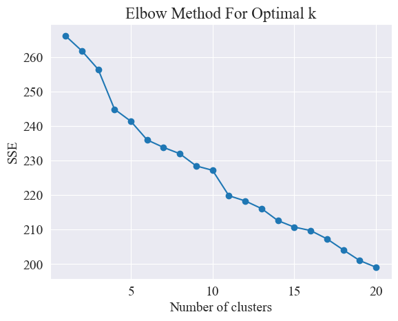
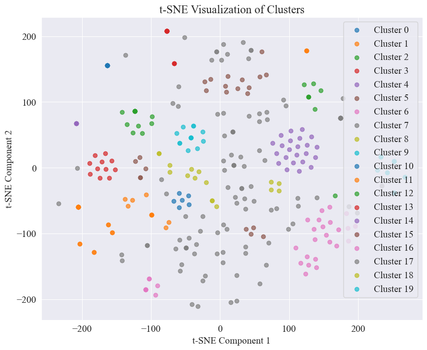
From the above figure, we determine that the clustering value of the elbow is 11, and draw the corresponding scatter plot. The results are as follows.
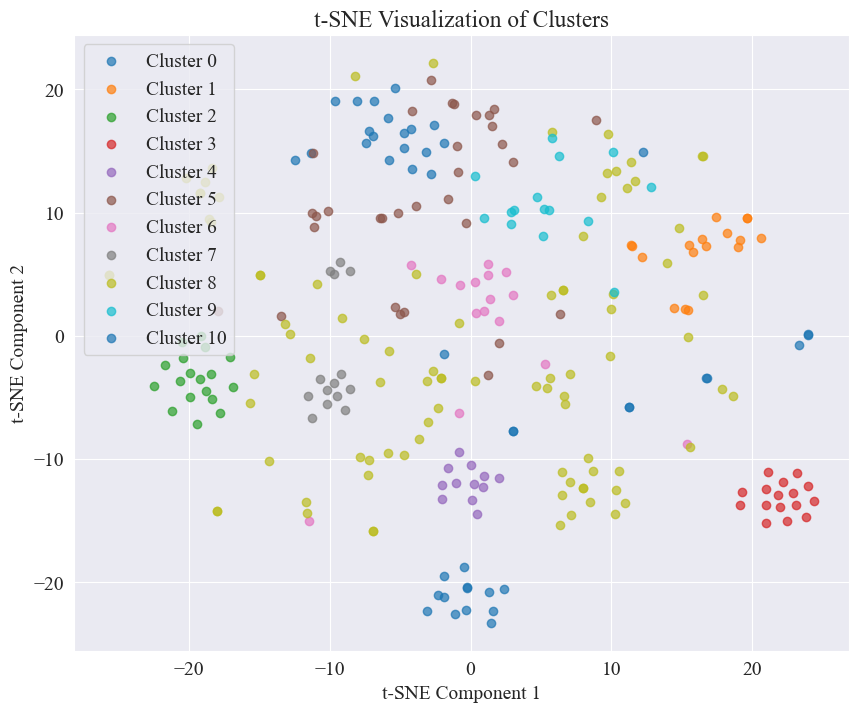
It can be seen that most of the rumor microblogs are well clustered, such as No. 3 and No. 4; some are widely distributed and not very well clustered, such as No. 5 and No. 8.
Clustering results
In order to clearly show which rumors are clustered in each class, a cloud map is drawn for each class. The results are as follows.
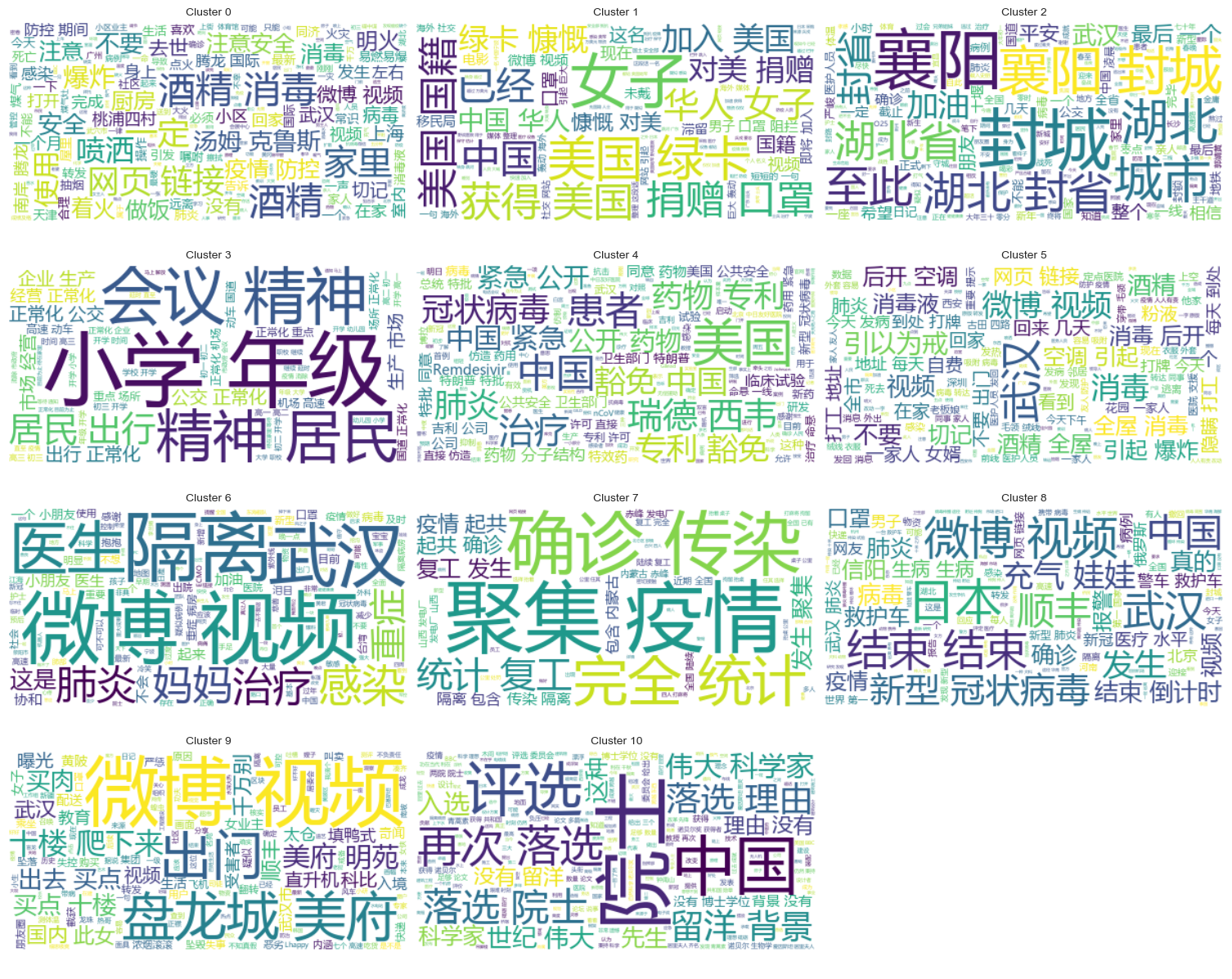
Print out some rumor microblog contents with better clustering, the results are as follows.
Cluster 2:
13    #封城日记#我的城市是湖北最后一个被封城的城市,金庸笔下的襄阳,郭靖黄蓉守城战死的地方。至此...
17    #襄阳封城#最后一座城被封,自此,湖北封省。在这大年三十夜。春晚正在说,为中国七十年成就喝彩...
18    #襄阳封城#过会襄阳也要封城了,到O25号0点,湖北省全省封省 ,希望襄阳的疑似患者能尽快确...
19    截止2020年1月25日00:00时❌湖北最后一个城市襄阳,整个湖北所有城市封城完毕,无公交...
21    #襄阳封城# 湖北省最后的一个城市于2020年1月25日零点零时零分正式封城至此,湖北省,封...
Name: rumorText, dtype: object

Cluster 3:
212    希望就在眼前…我期待着这一天早点到来。一刻都等不及了…西安学校开学时间:高三,初三,3月2日...
213    学校开学时间:高三,初三,3月2日开学,高一,高二,初一,初二,3月9日开学,小学4一6年级...
224    #长春爆料#【马上要解放了?真的假的?】长春学校开学时间:高三,初三,3月2日开学,高一,高...
225    有谁知道这是真的吗??我们这些被困湖北的外地人到底什么时候才能回家啊!(市政府会议精神,3月...
226    山东邹平市公布小道消息公布~:学校开学时间:高三,初三,3月2日开学,高一,高二,初一,初二...
Name: rumorText, dtype: object
Cluster analysis of rumor review results
Clustering rumor text content may not be effective for rumor content analysis, so we choose to cluster the rumor review results.
Determine the best cluster
Using the elbow plot, determine the best clustering.
From the above elbow diagram, we can identify two elbows, one when the cluster is 5 and the other when the cluster is 20. I choose 20 for clustering.
The scatter plot obtained by clustering 20 categories is as follows.
It can be seen that most of them are well clustered, but categories 7 and 17 are not well clustered.
Clustering results
In order to clearly show which rumor review results are clustered in each class, a cloud map is drawn for each class. The results are as follows.

Print out some rumor review results with better clustering, and the results are as follows.
Cluster 4:
52    从武汉撤回来的日本人,迎接他们的是每个人一台救护车,206人=206台救护车
53    从武汉撤回来的日本人,迎接他们的是每个人一台救护车,206人=206台救护车
54    从武汉撤回来的日本人,迎接他们的是每个人一台救护车,206人=206台救护车
55    从武汉撤回来的日本人,迎接他们的是每个人一台救护车,206人=206台救护车
56    从武汉撤回来的日本人,迎接他们的是每个人一台救护车,206人=206台救护车
Name: result, dtype: object

Cluster 10:
214    所有被啃噬、机化的肺组织都不会再恢复了,愈后会形成无任何肺功能的瘢痕组织
215    所有被啃噬、机化的肺组织都不会再恢复了,愈后会形成无任何肺功能的瘢痕组织
216    所有被啃噬、机化的肺组织都不会再恢复了,愈后会形成无任何肺功能的瘢痕组织
217    所有被啃噬、机化的肺组织都不会再恢复了,愈后会形成无任何肺功能的瘢痕组织
218    所有被啃噬、机化的肺组织都不会再恢复了,愈后会形成无任何肺功能的瘢痕组织
Name: result, dtype: object

Cluster 15:
7           在福州,里面坐的是周杰伦
8            周杰伦去福州自备隔离仓
9            周杰伦去福州自备隔离仓
10    周杰伦福州演唱会,给自己整了个隔离舱
12    周杰伦福州演唱会,给自己整了个隔离舱
Name: result, dtype: object
For this rumor detection, we chose to use a dataset that has been debunked. fact.json The similarity between the rumor debunked and the real rumor is compared, and the rumor debunking article with the highest similarity to the rumor microblog is selected as the basis for rumor detection.
Load Weibo rumor data and rumor refuting dataset
# 定义一个空的列表来存储每个 JSON 对象
fact_data = []

# 逐行读取 JSON 文件
with open('data/rumor/fact.json', 'r', encoding='utf-8') as f:
    for line in f:
        fact_data.append(json.loads(line.strip()))

# 创建辟谣数据的 DataFrame
fact_df = pd.DataFrame(fact_data)
fact_df = fact_df.dropna(subset=['title'])
Use a pre-trained language model to encode Weibo rumors and rumor-refuting titles into embedding vectors
This experiment used bert-base-chinese As a pre-trained model, model training is performed. The SimCSE model is used to improve the representation of sentence semantics and similarity measurement through contrastive learning.
# 加载SimCSE模型
model = SentenceTransformer('sentence-transformers/paraphrase-multilingual-MiniLM-L12-v2')
# 加载到 GPU
model.to('cuda')

# 加载预训练的NER模型
ner_pipeline = pipeline('ner', model='bert-base-chinese', aggregation_strategy="simple", device=0)
Calculating similarity
The similarity calculation uses the sentence embedding of the SimCSE model and the named entity similarity to calculate the comprehensive similarity.
extract_entitiesThe function uses the NER model to extract named entities in the text.
# 提取命名实体
def extract_entities(text):
    entities = ner_pipeline(text)
    return {entity['word'] for entity in entities}
entity_similarityThe function calculates the named entity similarity between two texts.
# 计算命名实体相似度
def entity_similarity(text1, text2):
    entities1 = extract_entities(text1)
    entities2 = extract_entities(text2)
    if not entities1 or not entities2:
        return 0.0
    intersection = entities1.intersection(entities2)
    union = entities1.union(entities2)
    return len(intersection) / len(union)
combined_similarityThe function combines the sentence embedding and named entity similarity of the SimCSE model to calculate the comprehensive similarity.
# 结合句子嵌入相似度和实体相似度
def combined_similarity(text1, text2):
    embed_sim = util.pytorch_cos_sim(model.encode([text1]), model.encode([text2])).item()
    entity_sim = entity_similarity(text1, text2)
    return 0.5 * embed_sim + 0.5 * entity_sim
Implementing rumor detection
By comparing similarities, the rumor detection mechanism is implemented.
def debunk_rumor(input_rumor):
    # 计算输入谣言与所有辟谣标题的相似度
    similarity_scores = []
    for fact_text in fact_df['title']:
        similarity_scores.append(combined_similarity(input_rumor, fact_text))

    # 找到最相似的辟谣标题
    most_similar_index = np.argmax(similarity_scores)
    most_similar_fact = fact_df.iloc[most_similar_index]

    # 输出辟谣判断及依据
    print("微博谣言:", input_rumor)
    print(f"辟谣判断:{most_similar_fact['explain']}")
    print(f"辟谣依据:{most_similar_fact['title']}")

weibo_rumor = "据最新研究发现,此次新型肺炎病毒传播途径是华南海鲜市场进口的豺——一种犬科动物携带的病毒,然后传给附近的狗,狗传狗,狗传人。狗不生病,人生病。人生病后又传给狗,循环传染。"
debunk_rumor(weibo_rumor)
The output is as follows:
微博谣言: 据最新研究发现,此次新型肺炎病毒传播途径是华南海鲜市场进口的豺——一种犬科动物携带的病毒,然后传给附近的狗,狗传狗,狗传人。狗不生病,人生病。人生病后又传给狗,循环传染。
辟谣判断:尚无定论
辟谣依据:狗能感染新型冠状病毒
Successfully find the basis for refuting the rumor and give a judgment on refuting the rumor.
Data Format
This experiment provides the epidemic-related news dataset CSDC-News, which collects news and commentary content in the first half of 2020. The dataset contains the following contents.
news
│
├─comment
│      01-01.txt
│      01-02.txt
...
│      03-08.txt
└─data
        01-01.txt
        01-02.txt
        ...
        08-31.txt
The data folder is divided into three parts:data,comment。
data The folder contains several files, each of which corresponds to data on a certain date in the formatjsonThe content of this part corresponds to the main text data of the news (which will be updated gradually with the date), and the fields include:
time: The time when the news was released.title: The title of the news.url:The original link of the news.meta: The main content of the news, including the following fields: content: The main content of the news.description: A short description of the news.title: The title of the news.keyword:News keywords.type: The type of news.comment The folder contains several files, each of which corresponds to data on a certain date in the formatjsonThe content in this section corresponds to the comment data of the news (there may be a delay of about one week between the comment data and the news text data). The fields include:
time: The time when the news was released, and data The data in the folder corresponds.title: The title of the news, and data The data in the folder corresponds.url: The original address link of the news, data The data in the folder corresponds.comment: News comment information. This field is an array. Each element of the array contains the following information: area: Commentator region.content:comments.nickname: Commentator's nickname.reply_to: The commenter’s reply object. If none, it means it is not a reply.time: Comment time.Data preprocessing
In the news article data data During data preprocessing, it is necessary tometa The contents in are released and stored in DataFrame format.
# 加载新闻数据
def load_news_data(data_dir):
    news_data = []
    files = sorted(os.listdir(data_dir))
    for file in files:
        if file.endswith('.txt'):
            with open(os.path.join(data_dir, file), 'r', encoding='utf-8') as f:
                daily_news = json.load(f)
                for news in daily_news:
                    news_entry = {
                        'time': news.get('time', 'NULL'),
                        'title': news.get('title', 'NULL'),
                        'url': news.get('url', 'NULL'),
                        'content': news.get('meta', {}).get('content', 'NULL'),
                        'description': news.get('meta', {}).get('description', 'NULL'),
                        'keyword': news.get('meta', {}).get('keyword', 'NULL'),
                        'meta_title': news.get('meta', {}).get('title', 'NULL'),
                        'type': news.get('meta', {}).get('type', 'NULL')
                    }
                    news_data.append(news_entry)
    return pd.DataFrame(news_data)
In the comment data comment During data preprocessing, it is necessary tocomment The contents in are released and stored in DataFrame format.
# 加载评论数据
def load_comment_data(data_dir):
    comment_data = []
    files = sorted(os.listdir(data_dir))
    for file in files:
        if file.endswith('.txt'):
            with open(os.path.join(data_dir, file), 'r', encoding='utf-8') as f:
                daily_comments = json.load(f)
                for comment in daily_comments:
                    for com in comment.get('comment', []):
                        comment_entry = {
                            'news_time': comment.get('time', 'NULL'),
                            'news_title': comment.get('title', 'NULL'),
                            'news_url': comment.get('url', 'NULL'),
                            'comment_area': com.get('area', 'NULL'),
                            'comment_content': com.get('content', 'NULL'),
                            'comment_nickname': com.get('nickname', 'NULL'),
                            'comment_reply_to': com.get('reply_to', 'NULL'),
                            'comment_time': com.get('time', 'NULL')
                        }
                        comment_data.append(comment_entry)
    return pd.DataFrame(comment_data)
Loading the dataset
According to the above data preprocessing function, load the dataset.
# 数据文件夹路径
news_data_dir = 'data/news/data/'
comment_data_dir = 'data/news/comment/'

# 加载数据
news_df = load_news_data(news_data_dir)
comment_df = load_comment_data(comment_data_dir)

# 展示加载的数据
print(f"新闻数据长度:{len(news_df)},评论数据:{len(comment_df)}")
The print result shows that the news data length is 502550 and the comment data length is 1534616.
News time distribution statistics
Separate statistics news_df The number of news articles per month and the number of news articles per hour are presented in bar charts and line charts. The results are as follows.
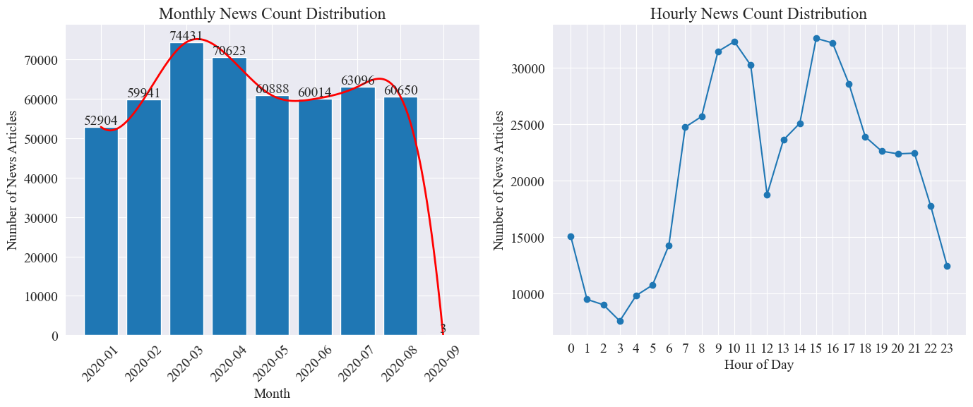
As can be seen from the above figure, with the outbreak of the epidemic, the number of news increased month by month, reaching a peak in March with 74,000 news articles, and then gradually declined to a stable level of 60,000 articles per month. Among them, the data in September was 3 articles at 0 o'clock, which can be excluded from the statistics.
According to the distribution of the number of news per hour, 10:00 and 15:00 are the peak times for news release, with more than 30,000 articles released each time. 12:00 is the lunch break, and the number of news releases shows a peak and valley. The number of news releases is the least from 0:00 to 5:00, with 3:00 being the smallest point.
News Hot Spot Tracking
This experiment intends to extract news keywords to track the news hot spots in the past 8 months. By counting the existing keyword distribution and drawing a bar chart, the results are as follows.
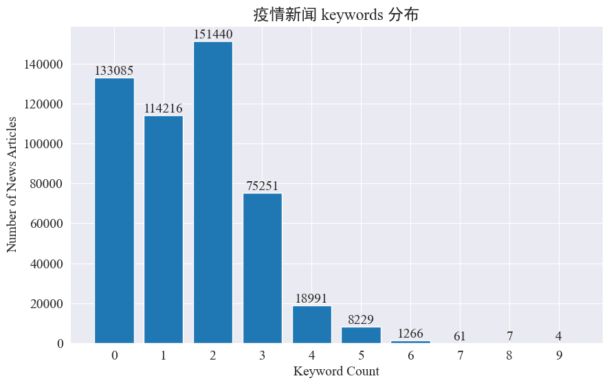
It can be seen that most news articles have less than 3 keywords, and even a large proportion of articles have no keywords. Therefore, it is necessary to summarize keywords by yourself for hot spot tracking. jieba.analyse.textrank() To count keywords.
import jieba
import jieba.analyse
def extract_keywords(text):
# 基于jieba的textrank算法实现
keywords = jieba.analyse.textrank(text,topK=5,withWeight=True)
return ' '.join([keyword[0] for keyword in keywords])
news_df['keyword_new'] =news_df['content'].map(lambda x: extract_keywords(x))
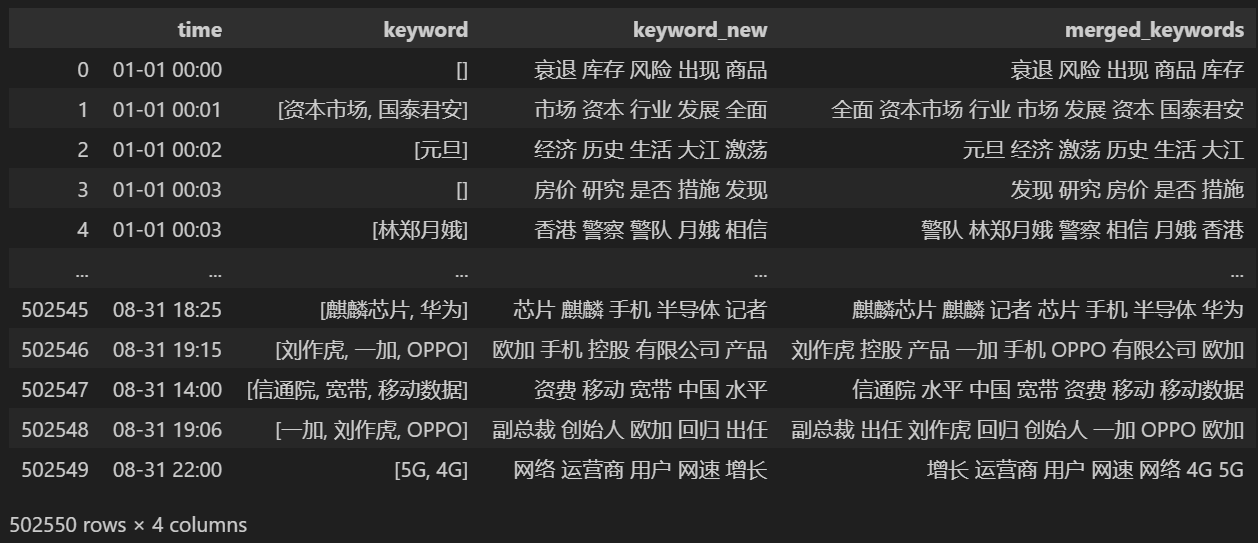
keyword_data = news_df[['time','keyword','keyword_new']]
keyword_data
Count 5 new keywords and store them in keyword_new, then merge keyword with them and remove duplicate words.
# 合并并去除重复的词
def merge_keywords(row):
    # 将keyword列和keyword_new列合并
    keywords = set(row['keyword']) | set(row['keyword_new'].split())
    return ' '.join(keywords)

keyword_data['merged_keywords'] = keyword_data.apply(merge_keywords, axis=1)
keyword_data
Merge and print keyword_data , the printed results are as follows.
In order to track hot spots, the frequency of all words that appear is counted and counted keyword_data['rolling_keyword_freq']。
# 按时间排序
keyword_data = keyword_data.sort_values(by='time')

# 计算滚动频率
def get_rolling_keyword_freq(df, window=7):
    rolling_keyword_freq = []
    for i in range(len(df)):
        start_time = df.iloc[i]['time'] - timedelta(days=window)
        end_time = df.iloc[i]['time']
        mask = (df['time'] > start_time) & (df['time'] <= end_time)
        recent_data = df.loc[mask]
        keywords = ' '.join(recent_data['merged_keywords']).split()
        keyword_counter = Counter(keywords)
        top_keywords = keyword_counter.most_common(20)
        rolling_keyword_freq.append(dict(top_keywords))
    return rolling_keyword_freq

keyword_data['rolling_keyword_freq'] = get_rolling_keyword_freq(keyword_data)

keyword_df = pd.DataFrame(keyword_data['rolling_keyword_freq'].tolist()).fillna(0)
keyword_df = keyword_df.astype(int)

# 将原始的时间列合并到新的DataFrame中
result_df = pd.concat([keyword_data['time'], keyword_df], axis=1)

# 保存为CSV文件
result_df.to_csv('./data/news/output/keyword_frequency.csv', index=False)
Then, based on the above statistical data, draw a chart showing the changes in hot words every day.
# 读取数据
file_path = './data/news/output/keyword_frequency.csv'
data = pd.read_csv(file_path, parse_dates=['time'])

# 聚合数据,按日期合并统计
data['date'] = data['time'].dt.date
daily_data = data.groupby('date').sum().reset_index()

# 准备颜色列表,确保每个关键词都有不同的颜色
colors = plt.cm.get_cmap('tab20', len(daily_data.columns[1:])).colors
color_dict = {keyword: colors[i] for i, keyword in enumerate(daily_data.columns[1:])}

def update(frame):
    plt.clf()
    date = daily_data['date'].iloc[frame]
    day_data = daily_data[daily_data['date'] == date].drop('date', axis=1).T
    day_data.columns = ['count']
    day_data = day_data.sort_values(by='count', ascending=False).head(10)

    bars = plt.barh(day_data.index, day_data['count'], color=[color_dict[keyword] for keyword in day_data.index])
    plt.xlabel('Count')
    plt.title(f'Keyword Frequency on {date}')
    for bar in bars:
        plt.text(bar.get_width(), bar.get_y() + bar.get_height()/2, f'{bar.get_width()}', va='center')
    plt.gca().invert_yaxis()

# 创建动画
fig = plt.figure(figsize=(10, 6))
anim = FuncAnimation(fig, update, frames=len(daily_data), repeat=False)

# 保存动画
anim.save('keyword_trend.gif', writer='imagemagick')
Finally, we get a gif of the changes in keywords in the epidemic news, and the results are as follows.
Before the outbreak, the terms "company" and "Iran" remained at high positions. After the outbreak, the number of news related to the epidemic soared in February, and then the term "new coronary pneumonia" soared and remained at the first position until the end of August, when the first wave of the epidemic slowed down and became the second.
This section first conducts a quantitative statistical analysis of news comments, and then conducts sentiment analysis on different comments.
Daily news comment statistics
Statistical trend of the number of news comments, expressed as a bar chart, and draw an approximate curve. The code is as follows.
# 提取日期和小时信息
dates = []
hours = []

for time_str in comment_df['news_time']:
    try:
        time_obj = datetime.strptime('2020-' + time_str, '%Y-%m-%d %H:%M')
        dates.append(time_obj.strftime('%Y-%m-%d'))
        hours.append(time_obj.hour)
    except ValueError:
        pass

# 统计每日新闻数量
daily_comment_counts = Counter(dates)
daily_comment_counts = dict(sorted(daily_comment_counts.items()))

# 统计每小时新闻数量
hourly_news_count = Counter(hours)
hourly_news_count = dict(sorted(hourly_news_count.items()))

# 绘制每月新闻数量分布柱状图
plt.figure(figsize=(14, 6))

days = list(daily_comment_counts.keys())
comment_counts = list(daily_comment_counts.values())
bars = plt.bar(days, comment_counts, label='Daily Comment Count')
plt.xlabel('Date')
plt.ylabel('Comment Count')
plt.title('Daily Comment Counts on News')
plt.xticks(rotation=80, fontsize=10)

# 绘制近似曲线
x = np.arange(len(days))
y = comment_counts
spl = UnivariateSpline(x, y, s=100)
xs = np.linspace(0, len(days) - 1, 500)
ys = spl(xs)
plt.plot(xs, ys, 'r', lw=2, label='Smoothed Curve')

plt.show()
The following is a statistical chart of the number of daily news comments.
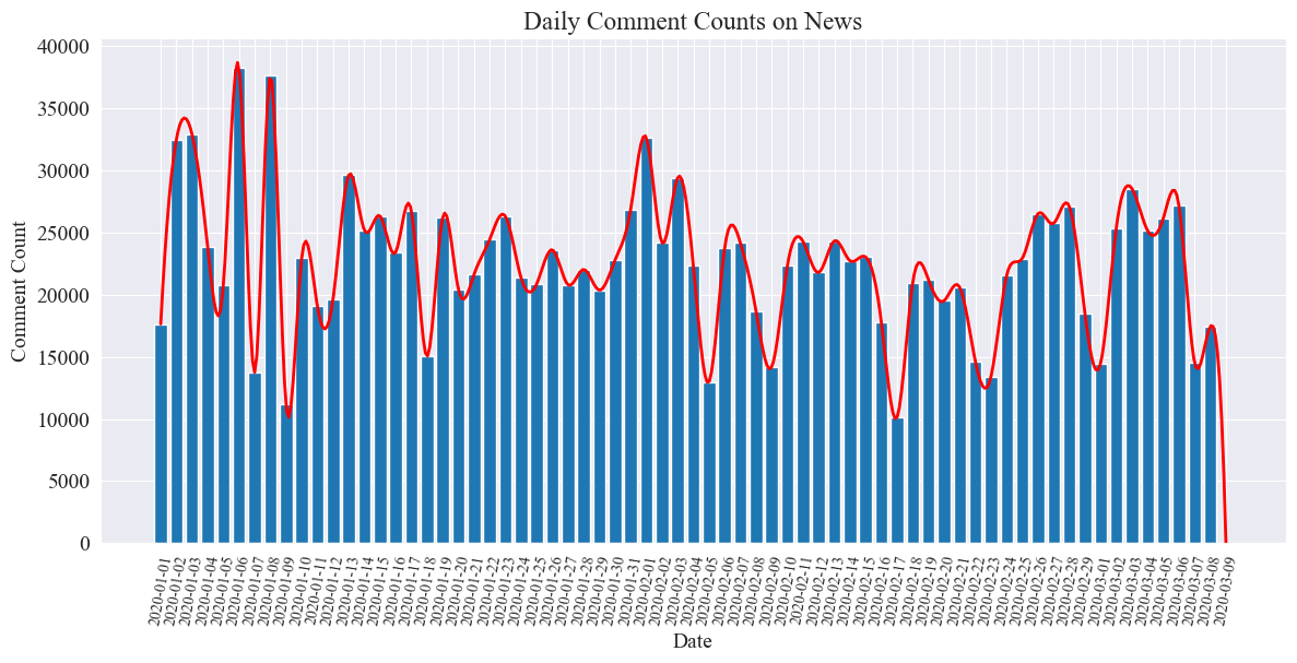
It can be seen that the number of news comments during the epidemic fluctuated between 10,000 and 40,000, with an average of about 20,000 comments per day.
Epidemic news by region
By province comment_df['province'] Count the number of news in each province, and count the number of comments on epidemic news in each province.
First, you need to pass comment_df['province'] Extract province information.
# 统计包含全国34个省、直辖市、自治区名称的地域数据
province_name = ['北京', '天津', '上海', '重庆', '河北', '河南', '云南', '辽宁', '黑龙江', '湖南', '安徽', '山东', '新疆',
                 '江苏', '浙江', '江西', '湖北', '广西', '甘肃', '山西', '内蒙古', '陕西', '吉林', '福建', '贵州', '广东',
                 '青海', '西藏', '四川', '宁夏', '海南', '台湾', '香港', '澳门']

# 提取省份信息
def extract_province(comment_area):
    for province in province_name:
        if province in comment_area:
            return province
    return None

comment_df['province'] = comment_df['comment_area'].apply(extract_province)

# 过滤出省份不为空的行
comment_df_filtered = comment_df[comment_df['province'].notnull()]

# 统计每个省份的评论数量
province_counts = comment_df_filtered['province'].value_counts().to_dict()
Then, based on the statistical data, a pie chart is drawn showing the proportion of news comments in each province.
# 计算总评论数量
total_comments = sum(province_counts.values())

# 计算各省份评论数量占比
provinces = []
comments = []
labels = []
for province, count in province_counts.items():
    if count / total_comments >= 0.02:
        provinces.append(province)
        comments.append(count)
        labels.append(province + f" ({count})")

# 绘制饼图
plt.figure(figsize=(10, 8))
plt.pie(comments, labels=labels, autopct='%1.1f%%', startangle=140)
plt.title('各省疫情新闻评论数量占比')
plt.axis('equal')  # 保证饼图是圆形
plt.show()

In this experiment, we also used pyecharts.charts ofMap Component, which plots the distribution of the number of comments by province on a map of China.
from pyecharts.charts import Map
from pyecharts import options as opts

# 省份简称到全称的映射字典
province_full_name = {
    '北京': '北京市',
    '天津': '天津市',
    '上海': '上海市',
    '重庆': '重庆市',
    '河北': '河北省',
    '河南': '河南省',
    '云南': '云南省',
    '辽宁': '辽宁省',
    '黑龙江': '黑龙江省',
    '湖南': '湖南省',
    '安徽': '安徽省',
    '山东': '山东省',
    '新疆': '新疆维吾尔自治区',
    '江苏': '江苏省',
    '浙江': '浙江省',
    '江西': '江西省',
    '湖北': '湖北省',
    '广西': '广西壮族自治区',
    '甘肃': '甘肃省',
    '山西': '山西省',
    '内蒙古': '内蒙古自治区',
    '陕西': '陕西省',
    '吉林': '吉林省',
    '福建': '福建省',
    '贵州': '贵州省',
    '广东': '广东省',
    '青海': '青海省',
    '西藏': '西藏自治区',
    '四川': '四川省',
    '宁夏': '宁夏回族自治区',
    '海南': '海南省',
    '台湾': '台湾省',
    '香港': '香港特别行政区',
    '澳门': '澳门特别行政区'
}

# 将省份名称替换为全称
full_province_counts = {province_full_name[key]: value for key, value in province_counts.items()}

# 创建中国地图
map_chart = (
    Map(init_opts=opts.InitOpts(width="1200px", height="800px"))
    .add("评论数量", [list(z) for z in zip(full_province_counts.keys(), full_province_counts.values())], "china")
    .set_global_opts(
        title_opts=opts.TitleOpts(title="中国各省疫情新闻评论数量分布"),
        visualmap_opts=opts.VisualMapOpts(max_=max(full_province_counts.values()))
    )
)

# 渲染图表为 HTML 文件
map_chart.render("comment_area_distribution.html")
In the obtained HTML, the distribution of the number of comments on epidemic news in each province of China is as follows.
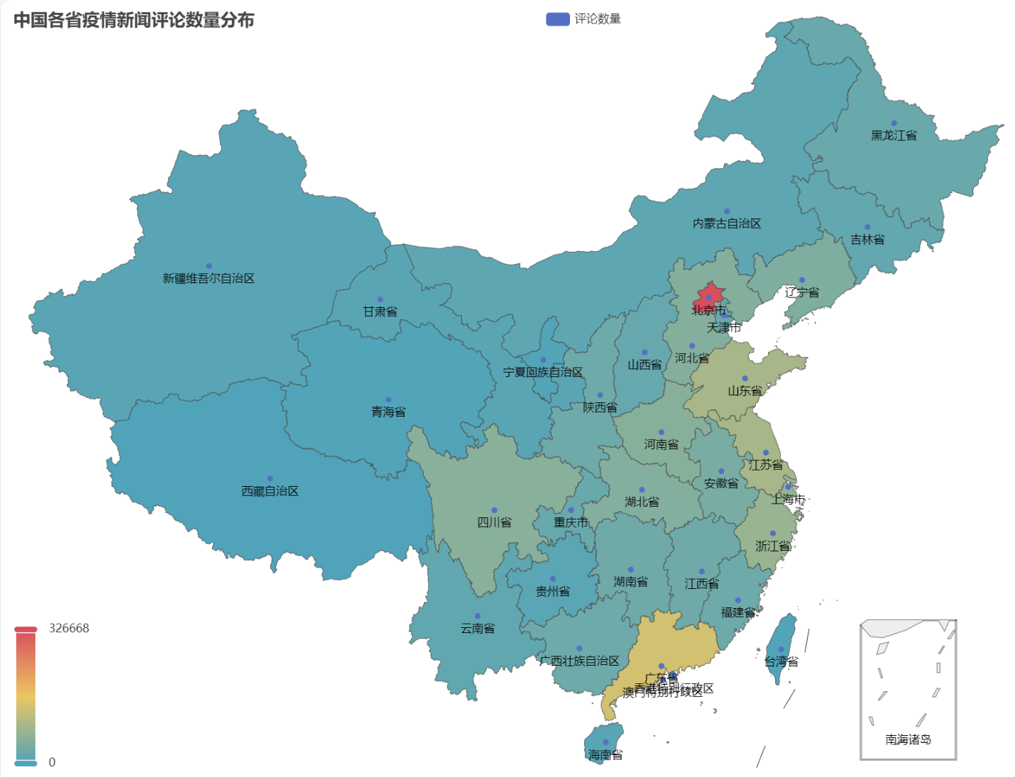
It can be seen that during the epidemic, the number of comments in Beijing accounted for the highest proportion, followed by Guangdong Province, and the number of comments in other provinces was relatively evenly distributed.
epidemicComment sentiment analysis
This experiment uses the NLP library for processing Chinese text SnowNLP , realize Chinese sentiment analysis, and give correspondingsentiment A value between 0 and 1, with values closer to 1 being more positive and closer to 0 being more negative.
from snownlp import SnowNLP

# 定义一个函数来计算情感得分,并处理可能的错误
def sentiment_analysis(text):
    try:
        s = SnowNLP(text)
        return s.sentiments
    except ZeroDivisionError:
        return None

# 对每条评论内容进行情感分析
comment_df['sentiment'] = comment_df['comment_content'].apply(sentiment_analysis)

# 删除情感得分为 None 的评论
comment_df = comment_df[comment_df['sentiment'].notna()]

# 将评论按正向(sentiment > 0.5)和负向(sentiment < 0.5)分类
comment_df['sentiment_label'] = comment_df['sentiment'].apply(lambda x: 'positive' if x > 0.5 else 'negative')
In this experiment, 0.5 is used as the threshold. Comments greater than this value are positive comments, and comments less than this value are negative comments. By writing code, a sentiment analysis chart of daily news comments is drawn, and the number of positive and negative comments of daily news is counted. The positive number is positive, and the negative number is negative.
# 提取新闻日期
comment_df['news_date'] = pd.to_datetime('2020-' + comment_df['news_time'].str[:5]).dt.date

# 统计每一天的正向和负向评论数量
daily_sentiment_counts = comment_df.groupby(['news_date', 'sentiment_label']).size().unstack(fill_value=0)

# 绘制柱状图
plt.figure(figsize=(14, 8))

# 绘制正向评论数量的柱状图
plt.bar(daily_sentiment_counts.index, daily_sentiment_counts['positive'], label='Positive', color='green')

# 绘制负向评论数量的柱状图(负数,以使其在 x 轴下方显示)
plt.bar(daily_sentiment_counts.index, -daily_sentiment_counts['negative'], label='Negative', color='red')

# 添加标签和标题
plt.xlabel('Date')
plt.ylabel('Number of Comments')
plt.title('Daily Sentiment Analysis of Comments')
plt.legend()

# 设置x轴刻度旋转
plt.xticks(rotation=45)

# 显示图表
plt.tight_layout()
plt.show()
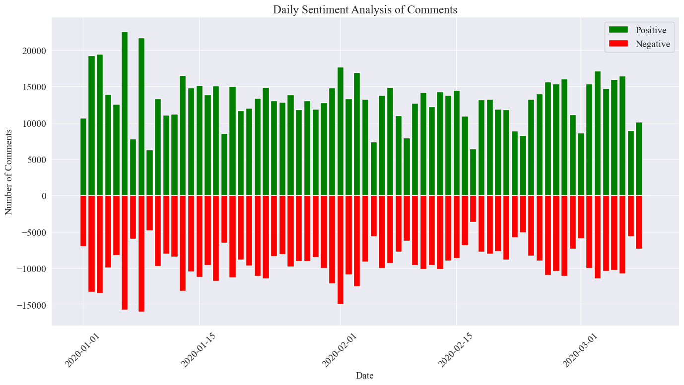
The final statistical image is as shown above. It can be seen that during the epidemic, positive comments were slightly higher than negative comments. By counting the proportion of positive comments, it was found that the proportion of positive comments was 58.63%, indicating that the public's attitude towards the epidemic was relatively positive.
Sentiment analysis of reviews by region
By counting the proportion of positive comments posted in each province and region, we obtained a chart showing the proportion of positive comments in each region.
# 计算各地区的积极评论数量和总评论数量
area_sentiment_stats = comment_df.groupby('province').agg(
    total_comments=('comment_content', 'count'),
    positive_comments=('sentiment', lambda x: (x > 0.5).sum())
)

# 计算各地区的积极评论占比
area_sentiment_stats['positive_ratio'] = area_sentiment_stats['positive_comments'] / area_sentiment_stats['total_comments']

# 绘制柱状图
plt.figure(figsize=(14, 7))
plt.bar(area_sentiment_stats.index, area_sentiment_stats['positive_ratio'], color='skyblue')
plt.xlabel('地区')
plt.ylabel('积极评论占比')
plt.title('各地区的积极评论占比')
plt.xticks(rotation=90)
plt.tight_layout()
plt.show()
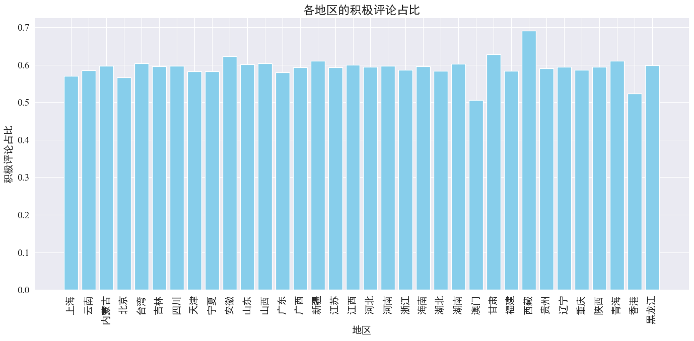
As can be seen from the above figure, the proportion of positive comments in most provinces is around 60%, among which Hong Kong and Macao have the lowest proportion of positive comments, about 50%, while Tibet has the highest proportion of positive comments, close to 70%.
From the above comment distribution, we can see that most comments from the mainland are positive, while negative comments from Hong Kong and Macao have increased significantly. Among them, Tibet has the highest number of positive comments, which may be due to the error caused by the small sample size in Tibet.
News Commentary Word Cloud Drawing
Word cloud diagrams of all comments, positive comments and negative comments are counted separately. In drawing the word cloud diagrams, positive comments are listed as above 0.6 and negative comments are listed as below 0.4. The following are three word cloud diagrams drawn.

It can be seen that most people's comments during the epidemic were relatively simple, such as "Haha", "good", etc. In the positive comments, we can see encouraging words such as "Go China" and "Go Wuhan", while in the negative comments, there are critical words such as "Hehe" and "Making money from the national disaster".

I have devoted myself to the research of technology for more than 30 years. I am proficient in various languages such as Java, Linux, JavaScript, PHP, CSS, etc. I have made many contributions in the field of open source. I have established a developer documentation site to share some problems in technology development for everyone to read.
