Shengsi 25-day learning card-punch camp day 23 | K nearest neighbor algorithm to achieve red wine clustering

Shengsi 25-day learning check-in camp day 23 | K nearest neighbor algorithm to achieve red wine clustering

2024-07-12

Can you win prizes by learning AI? 30 minutes a day, 25 days to open up AI's Ren and Du meridians (qq.com)

K-nearest neighbor algorithm for wine clustering

This experiment mainly introduces the use of MindSpore to conduct KNN experiments on some wine datasets.

1. Experimental purpose

Understand the basic concepts of KNN;
Learn how to use MindSpore to perform KNN experiments.

2. Introduction to the principle of K nearest neighbor algorithm

K-Nearest-Neighbor (KNN) is a nonparametric statistical method for classification and regression, originally proposed by Cover and Hart in 1968 (Cover et al., 1967), is one of the most basic algorithms for machine learning. It is based on the above idea: to determine the category of a sample, you can calculate its distance from all training samples, then find the k samples closest to the sample, count the categories of these samples and vote, and the class with the most votes is the classification result. The three basic elements of KNN are:

K value, the classification of a sample is determined by the "majority vote" of K neighbors. The smaller the K value, the easier it is to be affected by noise, and vice versa, the boundaries between categories will become blurred.
Distance metric reflects the similarity between two samples in the feature space. The smaller the distance, the more similar they are. Commonly used ones include Lp distance (when p=2, it is Euclidean distance), Manhattan distance, Hamming distance, etc.
The decision rule for classification is usually majority voting, or distance-weighted majority voting (with weights inversely proportional to distance).

Nonparametric statistical methods refer to statistical methods that do not rely on parametric forms (such as the normal distribution assumption in traditional statistics, etc.), that is, they do not have strict assumptions about the distribution of data. Compared with parametric statistical methods (such as linear regression, t-test, etc.), nonparametric statistical methods are more flexible because they do not assume that the data follows a specific distribution pattern.

Parametric statistical methods rely on specific assumptions and requirements for data distribution and describe the distribution of data through certain parameters. These parameterized forms can significantly simplify models and analysis, but they also require these assumptions and parameters to be consistent with actual data. When the assumptions are not met, misleading conclusions may result.
1. Linear Regression:
Assumption: There is a linear relationship between the dependent variable (response variable) and the independent variables (explanatory variables).
Parameters: regression coefficients (slope and intercept), usually assuming the error term has zero mean, constant variance (homoscedasticity), and a normal distribution.
2. Logistic Regression:
Assumption: The dependent variable (categorical variable) satisfies the logistic regression model and the regression coefficient is a fixed value.
Parameters: regression coefficients, which are used to describe the impact of the independent variables on the dependent variable and are estimated by maximum likelihood estimation.
3. t-test:
Assumption: The sample data comes from a normally distributed population.
Parameters: mean and variance, the one-sample t-test assumes the population mean, and the two-sample t-test assumes the difference between the means of the two populations.

2.1 Classification Problem

The flow of the prediction algorithm (classification) is as follows:

(1) Find the k samples closest to the test sample x_test in the training sample set and save them in the set N;

（2）统计集合N中每一类样本的个数𝐶𝑖,𝑖=1,2,3,...,𝑐；

（3）最终的分类结果为argmax𝐶𝑖 （最大的对应的𝐶𝑖）那个类。

In the above implementation process, the value of k is particularly important. It can be determined according to the problem and data characteristics. In the specific implementation, the weight of the sample can be considered, that is, each sample has a different voting weight. This method is called the weighted k-nearest neighbor algorithm, which is a variant of the k-nearest neighbor algorithm.

2.2 Regression Problem

假设离测试样本最近的k个训练样本的标签值为𝑦𝑖，则对样本的回归预测输出值为：

That is, the mean label of all neighbors.

The regression prediction function with sample weights is:

其中𝑤𝑖为第个𝑖样本的权重。

2.3 Definition of distance

KNN算法的实现依赖于样本之间的距离，其中最常用的距离函数就是欧氏距离（欧几里得距离）。ℝ𝑛空间中的两点𝑥和𝑦，它们之间的欧氏距离定义为：

It should be noted that when using Euclidean distance, each component of the eigenvector should be normalized to reduce the interference caused by the different scale ranges of the eigenvalues, otherwise the eigencomponents with small values will be overwhelmed by the eigencomponents with large values.

Other distance calculation methods include Mahalanobis distance, Bhattacharyya distance, etc.

3. Experimental environment

Prerequisites:

Proficiency in Python.
Have certain theoretical knowledge of machine learning, such as KNN, unsupervised learning, Euclidean distance, etc.

lab environment:

MindSpore 2.0 (MindSpore versions will be updated regularly, and this guide will also be updated regularly to match the version);
This case supports win_x86 and Linux systems, and can run on CPU/GPU/Ascend.
If you run this experiment locally, please refer to the MindSpore Environment Construction Experiment Manual to install MindSpore locally.

4. Data processing

4.1 Data Preparation

The Wine dataset is one of the most famous datasets for pattern recognition. The official website of the Wine dataset is:Wine Data SetThese data are the result of a chemical analysis of wines from the same region of Italy but from three different varieties. The dataset analyzes the amounts of 13 components contained in each of the three wines. These 13 properties are

Alcohol
Malic acid
Ash
Alcalinity of ash
Magnesium
Total phenols
Flavanoids
Nonflavanoid phenols
Proanthocyanins
Color intensity
Hue
OD280/OD315 of diluted wines
Proline

Method 1: Download from the Wine dataset official websitewine.data file。
Method 2: Download from HUAWEI CLOUD OBSwine.data file。

Key	Value	Key	Value
Data Set Characteristics:	Multivariate	Number of Instances:	178
Attribute Characteristics:	Integer, Real	Number of Attributes:	13
Associated Tasks:	Classification	Missing Values?	No


%%capture captured_output
# 实验环境已经预装了mindspore==2.2.14，如需更换mindspore版本，可更改下面mindspore的版本号
!pip uninstall mindspore -y
!pip install -i https://pypi.mirrors.ustc.edu.cn/simple mindspore==2.2.14


# 查看当前 mindspore 版本
!pip show mindspore

Name: mindspore
Version: 2.2.14
Summary: MindSpore is a new open source deep learning training/inference framework that could be used for mobile, edge and cloud scenarios.
Home-page: https://www.mindspore.cn
Author: The MindSpore Authors
Author-email: [email protected]
License: Apache 2.0
Location: /home/nginx/miniconda/envs/jupyter/lib/python3.9/site-packages
Requires: asttokens, astunparse, numpy, packaging, pillow, protobuf, psutil, scipy
Required-by:


from download import download
 
# 下载红酒数据集
url = "https://ascend-professional-construction-dataset.obs.cn-north-4.myhuaweicloud.com:443/MachineLearning/wine.zip"  
path = download(url, "./", kind="zip", replace=True)

Downloading data from https://ascend-professional-construction-dataset.obs.cn-north-4.myhuaweicloud.com:443/MachineLearning/wine.zip (4 kB)

file_sizes: 100%|██████████████████████████| 4.09k/4.09k [00:00<00:00, 2.51MB/s]
Extracting zip file...
Successfully downloaded / unzipped to ./

4.2 Data reading and processing

Import MindSpore modules and auxiliary modules

Before generating data, import the required Python libraries.

Currently, the os library is used. For ease of understanding, we will explain other required libraries when they are used specifically.

For detailed description of MindSpore modules, you can search and query on the MindSpore API page.

You can use context.set_context to configure the information required for operation, such as operation mode, backend information, hardware, etc.

Import the context module and configure the information required for running.


%matplotlib inline
import os
import csv
import numpy as np
import matplotlib.pyplot as plt
 
import mindspore as ms
from mindspore import nn, ops
 
ms.set_context(device_target="CPU")

refer tomindspore.set_context ，device_target(str) - Indicates the target device to be run, supporting 'Ascend', 'GPU' and 'CPU'. If this parameter is not set, the backend device corresponding to the MindSpore package is used. In the experimental environment, it can also be set to Ascend.

Reading Wine datasets`wine.data`, and view some of the data.


with open('wine.data') as csv_file:
    data = list(csv.reader(csv_file, delimiter=','))
print(data[56:62]+data[130:133])

[['1', '14.22', '1.7', '2.3', '16.3', '118', '3.2', '3', '.26', '2.03', '6.38', '.94', '3.31', '970'], ['1', '13.29', '1.97', '2.68', '16.8', '102', '3', '3.23', '.31', '1.66', '6', '1.07', '2.84', '1270'], ['1', '13.72', '1.43', '2.5', '16.7', '108', '3.4', '3.67', '.19', '2.04', '6.8', '.89', '2.87', '1285'], ['2', '12.37', '.94', '1.36', '10.6', '88', '1.98', '.57', '.28', '.42', '1.95', '1.05', '1.82', '520'], ['2', '12.33', '1.1', '2.28', '16', '101', '2.05', '1.09', '.63', '.41', '3.27', '1.25', '1.67', '680'], ['2', '12.64', '1.36', '2.02', '16.8', '100', '2.02', '1.41', '.53', '.62', '5.75', '.98', '1.59', '450'], ['3', '12.86', '1.35', '2.32', '18', '122', '1.51', '1.25', '.21', '.94', '4.1', '.76', '1.29', '630'], ['3', '12.88', '2.99', '2.4', '20', '104', '1.3', '1.22', '.24', '.83', '5.4', '.74', '1.42', '530'], ['3', '12.81', '2.31', '2.4', '24', '98', '1.15', '1.09', '.27', '.83', '5.7', '.66', '1.36', '560']]

取三类样本（共178条），将数据集的13个属性作为自变量𝑋。将数据集的3个类别作为因变量𝑌。¶


X = np.array([[float(x) for x in s[1:]] for s in data[:178]], np.float32)
Y = np.array([s[0] for s in data[:178]], np.int32)

By taking two attributes of the sample for 2D visualization, we can see the distribution and separability of the samples on the two attributes.


attrs = ['Alcohol', 'Malic acid', 'Ash', 'Alcalinity of ash', 'Magnesium', 'Total phenols',
         'Flavanoids', 'Nonflavanoid phenols', 'Proanthocyanins', 'Color intensity', 'Hue',
         'OD280/OD315 of diluted wines', 'Proline']
plt.figure(figsize=(10, 8))
for i in range(0, 4):
    plt.subplot(2, 2, i+1)
    a1, a2 = 2 * i, 2 * i + 1
    plt.scatter(X[:59, a1], X[:59, a2], label='1')
    plt.scatter(X[59:130, a1], X[59:130, a2], label='2')
    plt.scatter(X[130:, a1], X[130:, a2], label='3')
    plt.xlabel(attrs[a1])
    plt.ylabel(attrs[a2])
    plt.legend()
plt.show()

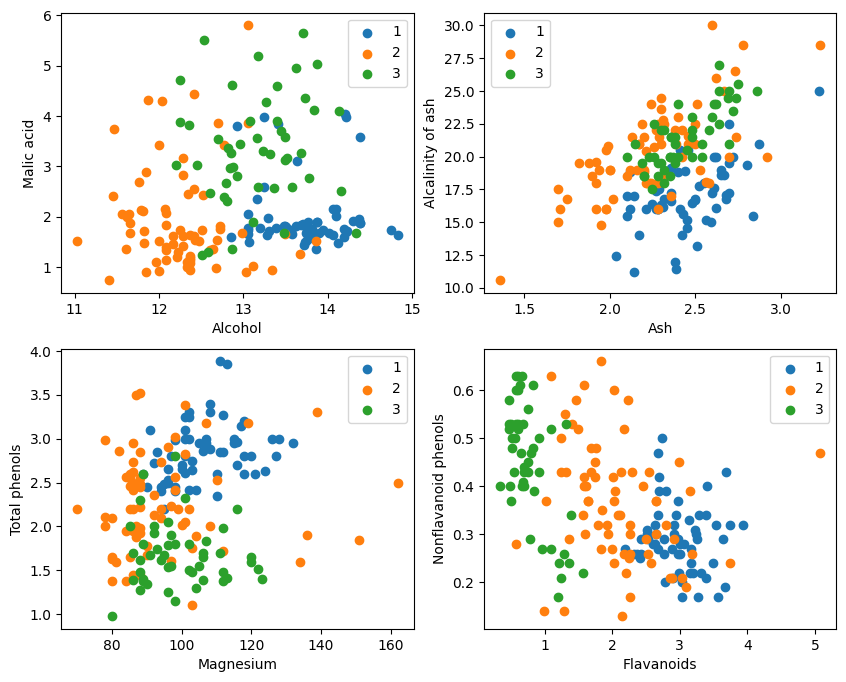
It is estimated from the code that the first 59 samples are probably of category 1, 59 to 130 are of category 2, and the rest are of category 3.

From the graphic display, the two attribute classification effects in the graphics in the upper left corner and the lower right corner are better, especially the boundary between category 1 and category 2 is more obvious.

The dataset is divided into a training set (known category samples) and a validation set (samples to be verified) at a ratio of 128:50:¶


train_idx = np.random.choice(178, 128, replace=False)
test_idx = np.array(list(set(range(178)) - set(train_idx)))
X_train, Y_train = X[train_idx], Y[train_idx]
X_test, Y_test = X[test_idx], Y[test_idx]

分解test_idx = np.array(list(set(range(178)) - set(train_idx)))
1. range(178) generates a sequence of integers from 0 to 177.
2. set(range(178)) converts this integer sequence into a set. A set is a data structure that does not allow duplicate elements and supports efficient set operations (such as union, intersection, and difference).
3. set(train_idx) converts the randomly selected training set index list train_idx into a set.
4. set(range(178)) - set(train_idx) calculates the difference of the sets and obtains the elements in set(range(178)) but not in set(train_idx), which are the indices of the test set. This is a set operation that can quickly and efficiently calculate the difference elements.
5. list(...) converts the result of the difference operation back into a list.
6. np.array(...) converts this list into a numpy array so that it can be indexed with numpy arrays X and Y。

5. Model construction-calculating distance

Using MindSporetile, square, ReduceSum, sqrt, TopKOperators such as , use matrix operations to simultaneously calculate the distance between the input sample x and other clearly classified samples X_train, and calculate the top k nearest neighbors


class KnnNet(nn.Cell):
    def __init__(self, k):
        super(KnnNet, self).__init__()
        self.k = k
 
    def construct(self, x, X_train):
        #平铺输入x以匹配X_train中的样本数
        x_tile = ops.tile(x, (128, 1))
        square_diff = ops.square(x_tile - X_train)
        square_dist = ops.sum(square_diff, 1)
        dist = ops.sqrt(square_dist)
        #-dist表示值越大，样本就越接近
        values, indices = ops.topk(-dist, self.k)
        return indices
 
def knn(knn_net, x, X_train, Y_train):
    x, X_train = ms.Tensor(x), ms.Tensor(X_train)
    indices = knn_net(x, X_train)
    topk_cls = [0]*len(indices.asnumpy())
    for idx in indices.asnumpy():
        topk_cls[Y_train[idx]] += 1
    cls = np.argmax(topk_cls)
    return cls

1. Define the KNN network class: KnnNet
__init__ function: initialize the network and set the K value (that is, the number of nearest neighbors selected).
construct function: Calculates the Euclidean distance between the input sample x and each sample in the training set X_train, and returns the index of the k samples with the smallest distance (i.e., the nearest neighbor).
2. Define KNN function: knn
Receives knn_net (KNN network instance), test sample x, training sample X_train and training labels Y_train as input.
Use knn_net to find the k nearest neighbor samples of x, classify them according to the labels of these samples, and return the classification results (i.e. the predicted categories).

6. Model prediction

在验证集上验证KNN算法的有效性，取𝑘=5，验证精度接近80%，说明KNN算法在该3分类任务上有效，能根据酒的13种属性判断出酒的品种。


acc = 0
knn_net = KnnNet(5)
for x, y in zip(X_test, Y_test):
    pred = knn(knn_net, x, X_train, Y_train)
    acc += (pred == y)
    print('label: %d, prediction: %s' % (y, pred))
print('Validation accuracy is %f' % (acc/len(Y_test)))

Calculate and print the accuracy of the test set
Loop through each sample in the test set X_test and Y_test, and use the knn function to classify each sample.
Count the number of samples that are correctly predicted, calculate and output the classification accuracy.

label: 1, prediction: 1
label: 2, prediction: 3
label: 1, prediction: 1
label: 1, prediction: 1
label: 3, prediction: 2
label: 1, prediction: 1
label: 1, prediction: 1
label: 3, prediction: 3
label: 1, prediction: 1
label: 1, prediction: 1
label: 1, prediction: 1
label: 1, prediction: 1
label: 3, prediction: 2
label: 1, prediction: 2
label: 1, prediction: 1
label: 1, prediction: 1
label: 3, prediction: 2
label: 1, prediction: 1
label: 1, prediction: 1
label: 3, prediction: 3
label: 3, prediction: 1
label: 3, prediction: 2
label: 3, prediction: 2
label: 1, prediction: 1
label: 1, prediction: 1
label: 3, prediction: 2
label: 1, prediction: 3
label: 3, prediction: 1
label: 3, prediction: 3
label: 3, prediction: 1
label: 3, prediction: 1
label: 1, prediction: 1
label: 1, prediction: 1
label: 1, prediction: 1
label: 1, prediction: 1
label: 2, prediction: 2
label: 2, prediction: 2
label: 2, prediction: 3
label: 2, prediction: 3
label: 2, prediction: 2
label: 2, prediction: 2
label: 2, prediction: 2
label: 2, prediction: 1
label: 2, prediction: 3
label: 2, prediction: 2
label: 2, prediction: 2
label: 2, prediction: 2
label: 2, prediction: 2
label: 2, prediction: 2
label: 2, prediction: 2
Validation accuracy is 0.660000

It is not possible to reach 80% every time. After trying many times, I finally got the accuracy to 80% once:

label: 1, prediction: 1
label: 3, prediction: 3
label: 1, prediction: 1
label: 1, prediction: 1
label: 3, prediction: 3
label: 3, prediction: 3
label: 3, prediction: 2
label: 3, prediction: 3
label: 1, prediction: 1
label: 3, prediction: 3
label: 1, prediction: 1
label: 1, prediction: 3
label: 3, prediction: 3
label: 1, prediction: 3
label: 1, prediction: 1
label: 3, prediction: 3
label: 1, prediction: 1
label: 1, prediction: 1
label: 3, prediction: 3
label: 3, prediction: 3
label: 3, prediction: 2
label: 1, prediction: 1
label: 3, prediction: 3
label: 1, prediction: 1
label: 3, prediction: 3
label: 1, prediction: 1
label: 1, prediction: 1
label: 1, prediction: 1
label: 1, prediction: 1
label: 1, prediction: 1
label: 1, prediction: 1
label: 1, prediction: 1
label: 2, prediction: 3
label: 2, prediction: 1
label: 2, prediction: 2
label: 2, prediction: 2
label: 2, prediction: 2
label: 2, prediction: 2
label: 2, prediction: 3
label: 2, prediction: 2
label: 2, prediction: 2
label: 2, prediction: 2
label: 2, prediction: 3
label: 2, prediction: 2
label: 2, prediction: 2
label: 2, prediction: 2
label: 2, prediction: 2
label: 2, prediction: 2
label: 2, prediction: 3
label: 2, prediction: 2
Validation accuracy is 0.820000

Experimental Summary

This experiment uses MindSpore to implement the KNN algorithm to solve the 3-classification problem. Take the 3 types of samples in the wine dataset and divide them into known category samples and to-be-verified samples. From the verification results, it can be seen that the KNN algorithm is effective in this task and can determine the type of wine based on the 13 attributes of the wine.

Data preparation: Download data from the Wine dataset official website or Huawei Cloud OBS for reading and processing.

Data processing: The dataset is divided into independent variables (13 attributes) and dependent variables (3 categories), and visualization is performed to observe the sample distribution.

Model construction: Define the KNN network structure, use the operators provided by MindSpore to calculate the distance between the input sample and the training sample, and find the nearest k neighbors.

Model prediction: Make predictions on the validation set and calculate the prediction accuracy.

Experimental results show that the classification accuracy of the KNN algorithm on the Wine dataset is close to 80% (66%).

Technology Sharing

Shengsi 25-day learning check-in camp day 23 | K nearest neighbor algorithm to achieve red wine clustering

K-nearest neighbor algorithm for wine clustering

1. Experimental purpose

2. Introduction to the principle of K nearest neighbor algorithm

2.1 Classification Problem

2.2 Regression Problem

2.3 Definition of distance

3. Experimental environment

4. Data processing

4.1 Data Preparation

4.2 Data reading and processing

Import MindSpore modules and auxiliary modules

refer tomindspore.set_context ，device_target(str) - Indicates the target device to be run, supporting 'Ascend', 'GPU' and 'CPU'. If this parameter is not set, the backend device corresponding to the MindSpore package is used. In the experimental environment, it can also be set to Ascend.

Reading Wine datasets`wine.data`, and view some of the data.

取三类样本（共178条），将数据集的13个属性作为自变量𝑋。将数据集的3个类别作为因变量𝑌。¶

By taking two attributes of the sample for 2D visualization, we can see the distribution and separability of the samples on the two attributes.

It is estimated from the code that the first 59 samples are probably of category 1, 59 to 130 are of category 2, and the rest are of category 3.

The dataset is divided into a training set (known category samples) and a validation set (samples to be verified) at a ratio of 128:50:¶

5. Model construction-calculating distance

6. Model prediction

Experimental Summary

Personal profile

my contact information

Technology Sharing

Shengsi 25-day learning check-in camp day 23 | K nearest neighbor algorithm to achieve red wine clustering

K-nearest neighbor algorithm for wine clustering

1. Experimental purpose

2. Introduction to the principle of K nearest neighbor algorithm

2.1 Classification Problem

2.2 Regression Problem

2.3 Definition of distance

3. Experimental environment

4. Data processing

4.1 Data Preparation

4.2 Data reading and processing

Import MindSpore modules and auxiliary modules

refer tomindspore.set_context ，device_target(str) - Indicates the target device to be run, supporting 'Ascend', 'GPU' and 'CPU'. If this parameter is not set, the backend device corresponding to the MindSpore package is used. In the experimental environment, it can also be set to Ascend.

Reading Wine datasetswine.data, and view some of the data.

取三类样本（共178条），将数据集的13个属性作为自变量𝑋。将数据集的3个类别作为因变量𝑌。¶

By taking two attributes of the sample for 2D visualization, we can see the distribution and separability of the samples on the two attributes.

It is estimated from the code that the first 59 samples are probably of category 1, 59 to 130 are of category 2, and the rest are of category 3.

The dataset is divided into a training set (known category samples) and a validation set (samples to be verified) at a ratio of 128:50:¶

5. Model construction-calculating distance

6. Model prediction

Experimental Summary

Personal profile

my contact information

Reading Wine datasets`wine.data`, and view some of the data.