Technology Sharing

한어Русский языкEnglishFrançaisIndonesianSanskrit日本語DeutschPortuguêsΕλληνικάespañolItalianoSuomalainenLatina

Summary

This article comprehensively reviews the development of activation functions in deep learning, from the early Sigmoid and Tanh functions to the widely used ReLU series, and then to the recently proposed new activation functions such as Swish, Mish and GeLU. The mathematical expressions, characteristics, advantages, limitations and applications of various activation functions in typical models are deeply analyzed. Through systematic comparative analysis, this article explores the design principles, performance evaluation criteria and possible future development directions of activation functions, providing theoretical guidance for the optimization and design of deep learning models.

1 Introduction

The activation function is a key component in the neural network. It introduces nonlinear characteristics at the output of the neuron, enabling the neural network to learn and represent complex nonlinear mappings. Without the activation function, no matter how deep the neural network is, it can only represent linear transformations in essence, which greatly limits the network's expressive power.
With the rapid development of deep learning, the design and selection of activation functions have become an important factor affecting model performance. Different activation functions have different characteristics, such as gradient fluidity, computational complexity, degree of nonlinearity, etc. These characteristics directly affect the training efficiency, convergence speed and final performance of the neural network.
This article aims to comprehensively review the evolution of activation functions, deeply analyze the characteristics of various activation functions, and explore their applications in modern deep learning models. We will discuss the following aspects:

1. Classic activation functions: including Sigmoid, Tanh and other commonly used activation functions in the early days.
2. ReLU and its variants: including ReLU, Leaky ReLU, PReLU, ELU, etc.
3. New activation functions: such as Swish, Mish, GeLU and other recently proposed functions.
4. Special-purpose activation functions: such as Softmax, Maxout, etc.
5. Comparison and selection of activation functions: Discuss the selection strategies of activation functions in different scenarios.
6. Future Outlook: Explore possible development directions of activation function research.

Through this systematic review and analysis, we hope to provide a comprehensive reference for researchers and practitioners to help them better choose and use activation functions in deep learning model design.

2. Classic activation function

2.1 Sigmoid function

The Sigmoid function is one of the earliest widely used activation functions, and its mathematical expression is:
$\sigma (x)=\frac{1}{1+e^{-x}}$

Features and Benefits:

1. Output range is bounded: The output range of the Sigmoid function is between (0, 1), which makes it particularly suitable for dealing with probability problems.
2. Smooth and drivable: The function is smooth and differentiable in the entire domain, which is conducive to the application of the gradient descent algorithm.
3. Strong explanation: The output can be interpreted as a probability, which is particularly suitable for the output layer of a binary classification problem.

Disadvantages and limitations:

1. Vanishing Gradient Problem: When the input value is very large or very small, the gradient is close to zero, which leads to the gradient vanishing problem in deep networks.
2. Output non-zero center: The outputs of Sigmoid are all positive, which may cause the input of the next layer of neurons to always be positive, affecting the convergence speed of the model.
3. Computational complexity: It involves exponential operations and the computational complexity is relatively high.

Applicable scene:

1. Early shallow neural networks.
2. Output layer for binary classification problem.
3. Scenarios where the output needs to be limited to the range (0, 1).

Comparison with other functions:

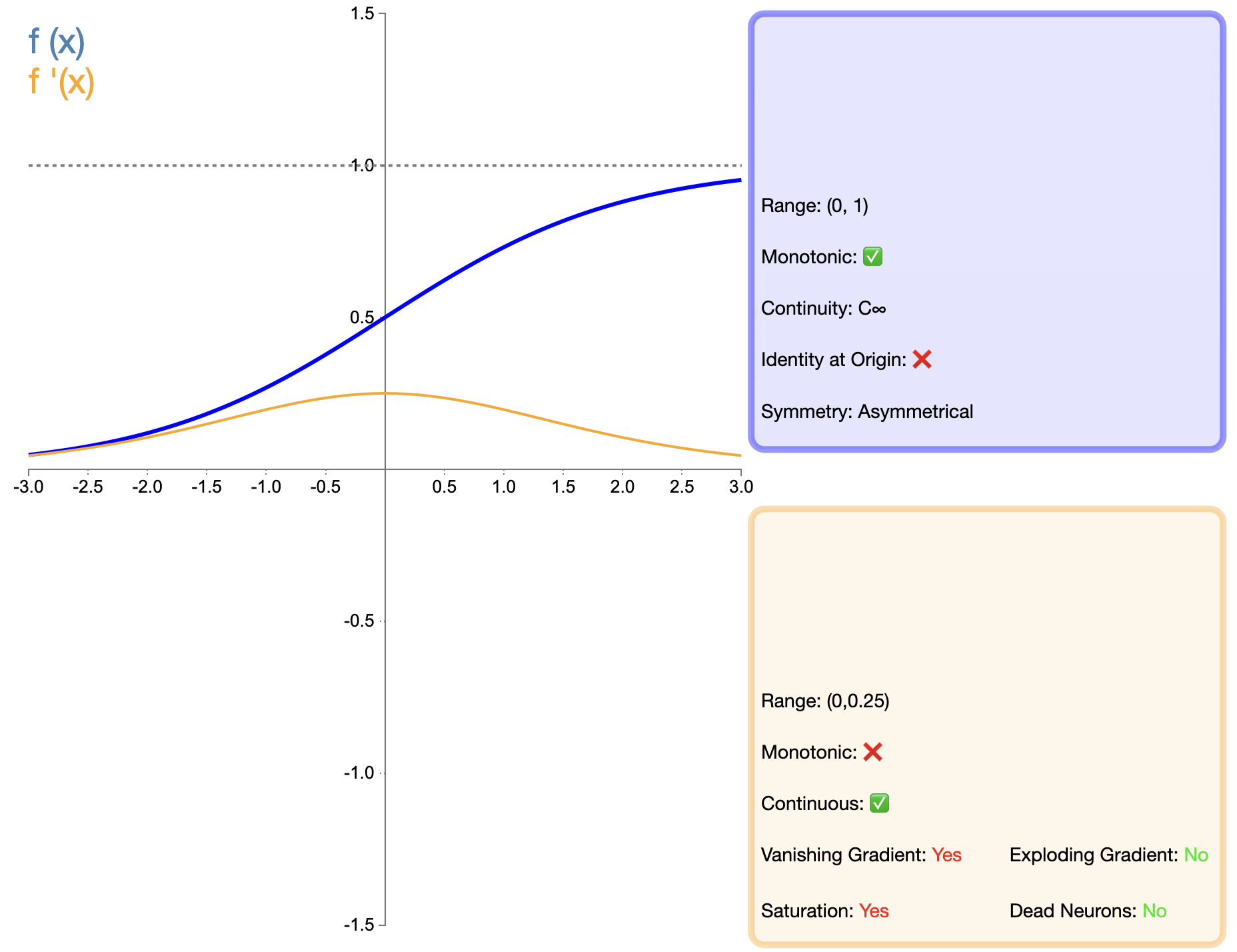
Compared with the later functions such as ReLU, the application of Sigmoid in deep networks is greatly limited, mainly because of its gradient vanishing problem. However, in some specific tasks (such as binary classification), Sigmoid is still an effective choice.

2.2 Tanh function

The Tanh (hyperbolic tangent) function can be regarded as an improved version of the Sigmoid function, and its mathematical expression is:
$\tanh (x)=\frac{e^x-e^{-x}}{e^x+e^{-x}}$

Features and Benefits:

1. Zero center output: The output range of the Tanh function is between (-1, 1), which solves the non-zero center problem of Sigmoid.
2. Stronger gradient: In the area where the input is close to zero, the gradient of the Tanh function is larger than that of the Sigmoid function, which helps to speed up learning.
3. Smooth and drivable: Similar to Sigmoid, Tanh is also smooth and differentiable.

Disadvantages and limitations:

1. Vanishing Gradient Problem: Although it is an improvement over Sigmoid, Tanh still has the problem of gradient vanishing when the input value is large or small.
2. Computational complexity: Similar to Sigmoid, Tanh also involves exponential operations and has a higher computational complexity.

Applicable scene:

1. It is better than Sigmoid in scenarios where zero-centered output is required.
2. It is often used in recurrent neural networks (RNNs) and long short-term memory networks (LSTMs).
3. Used in some scenarios where normalized output is important.

Improvements and comparisons:

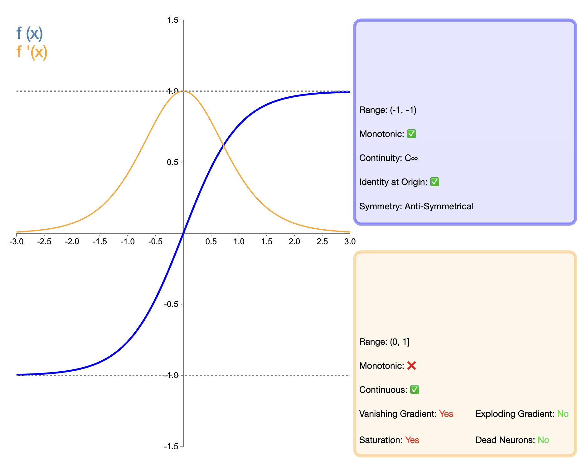
The Tanh function can be seen as an improved version of the Sigmoid function, with the main improvement being the zero-centering of the output. This feature makes Tanh perform better than Sigmoid in many cases, especially in deep networks. However, compared to later functions such as ReLU, Tanh still has the problem of gradient vanishing, which may affect the performance of the model in very deep networks.
Sigmoid and Tanh, two classic activation functions, played an important role in the early days of deep learning. Their characteristics and limitations also promoted the development of subsequent activation functions. Although they have been replaced by newer activation functions in many scenarios, they still have their unique application value in specific tasks and network structures.

3. ReLU and its variants

3.1 ReLU (Rectified Linear Unit)

The introduction of the ReLU function is an important milestone in the development of activation functions. Its mathematical expression is simple:
$\text{ReLU}(x)=\max (0,x)$

Features and Benefits:

1. Simple calculation: The computational complexity of ReLU is much lower than that of Sigmoid and Tanh, which is conducive to accelerating network training.
2. Alleviating gradient vanishing: For positive input, the gradient of ReLU is always 1, which effectively alleviates the gradient vanishing problem in deep networks.
3. Sparse Activation: ReLU can make the output of some neurons 0, resulting in sparse expression of the network, which is beneficial in some tasks.
4. Biological explanation: The unilateral inhibition property of ReLU is similar to the behavior of biological neurons.

Disadvantages and limitations:

1. The "Dead ReLU" Problem: When the input is negative, the gradient is zero, which may cause the neuron to be permanently inactivated.
2. Non-zero center output: The outputs of ReLU are all non-negative values, which may affect the learning process of the next layer.

Applicable scene:

1. Widely used in deep convolutional neural networks (such as ResNet, VGG).
2. Applicable to most feed-forward neural networks.

Comparison with other functions:

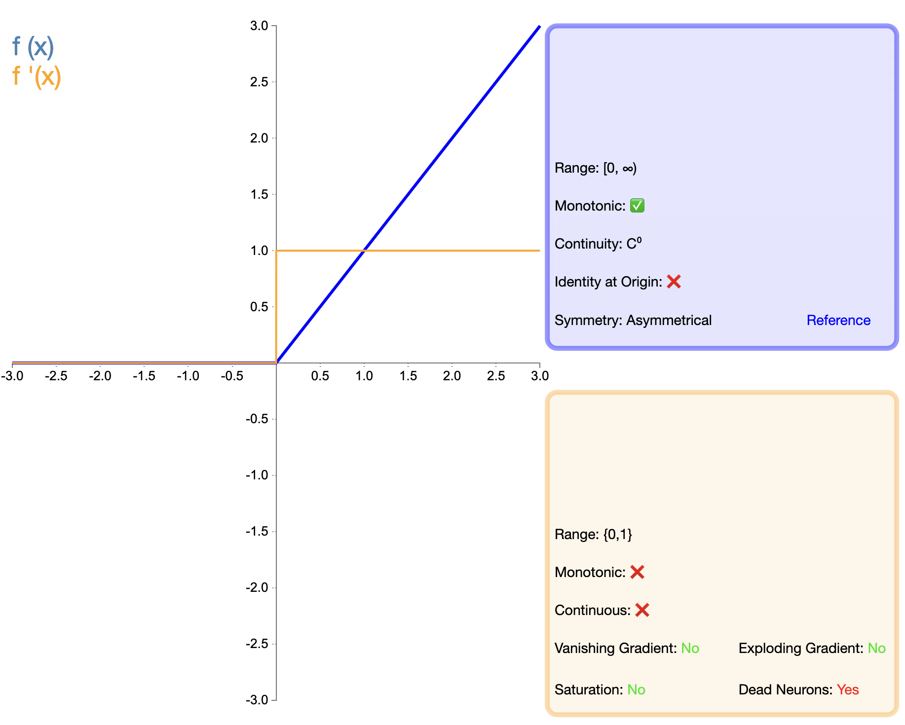
Compared with Sigmoid and Tanh, ReLU has shown significant advantages in deep networks, mainly in terms of training speed and alleviating gradient disappearance. However, the "dead ReLU" problem has prompted researchers to propose a variety of improved versions.

3.2 Leaky ReLU

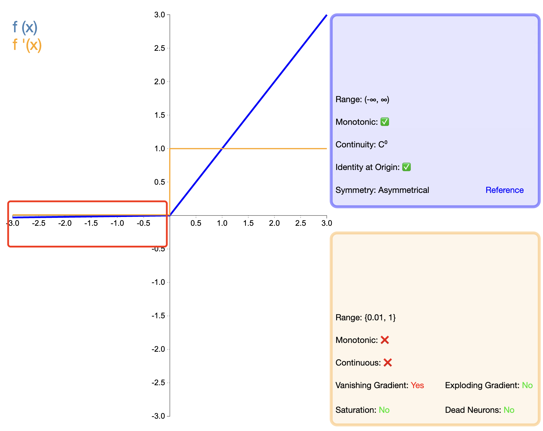
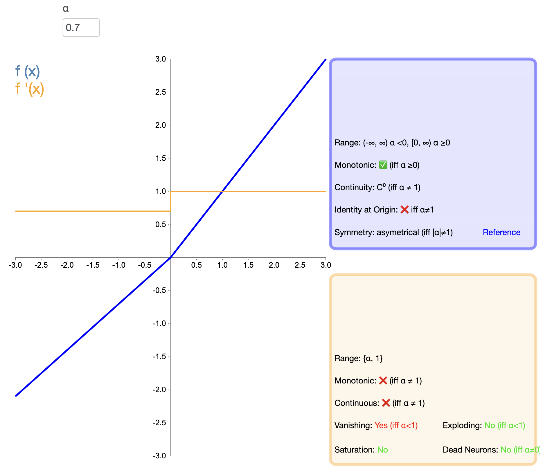
In order to solve the "death" problem of ReLU, Leaky ReLU was proposed:
$\text{Leaky ReLU}(x)=\{\begin{array}{ll}x,& \text{if }x>0\\ \alpha x,& \text{if }x\le 0\end{array}$
in,$\alpha$ is a small positive constant, usually 0.01.

Features and Benefits:

1. Alleviating the "Dead ReLU" Problem: When the input is negative, a small gradient is still retained to prevent the neuron from being completely inactivated.
2. Keep the advantages of ReLU：Maintaining linearity on the positive semi-axis, simple calculation, and helping to alleviate gradient disappearance.

Disadvantages and limitations:

1. Introducing hyperparameters：$\alpha$The choice of value requires tuning, which increases the complexity of the model.
2. Non-zero center output: Similar to ReLU, the output is still not zero-centered.

Applicable scene:

1. As an alternative in scenarios where ReLU performs poorly.
2. Used in tasks where some negative value information needs to be preserved.

3.3 PReLU (Parametric ReLU)

PReLU is a variant of Leaky ReLU, where the slope of the negative axis is a learnable parameter:
$\text{PReLU}(x)=\{\begin{array}{ll}x,& \text{if }x>0\\ \alpha x,& \text{if }x\le 0\end{array}$
here$\alpha$ are the parameters learned through back-propagation.

Features and Benefits:

1. Adaptive Learning: The most suitable negative semi-axis slope can be automatically learned based on the data.
2. Performance potential: In some tasks, PReLU can achieve better performance than ReLU and Leaky ReLU.

Disadvantages and limitations:

1. Increasing model complexity: The introduction of additional learnable parameters increases the complexity of the model.
2. Possible overfitting: In some cases, it may lead to overfitting, especially on small datasets.

Applicable scene:

1. Deep learning tasks on large-scale datasets.
2. Scenarios where adaptive activation functions are needed.

3.4 ELU (Exponential Linear Unit)

ELU attempts to combine the advantages of ReLU and the processing of negative inputs. Its mathematical expression is:
$\text{ELU}(x)=$